


Section I: Brief Introduction on AdaLine
The key difference between the AdaLine rule and Rosenblatt’s perceptron is that the weights are updated based on a linear activation function rather than a unit step function like in the perceptron. More specifically, the AdaLine algorithm compares the true class labels with the linear activation function’s continuous valued output to compute the model error and update the weights. In contrast, the perceptron compares the true class labels to the predicted class labels.
Section II: Code Snipet
方式一:基于批处理梯度下降模式的AdaLine实现
import numpy as np

class AdalineGD(object):
    def __init__(self,eta=0.01,n_iter=50,random_state=1):
        self.eta=eta
        self.n_iter=n_iter
        self.random_state=random_state

    def fit(self,X,y):
        rgen=np.random.RandomState(self.random_state)
        self.w_=rgen.normal(loc=0.0,scale=0.01,size=1+X.shape[1])
        self.cost_=[]

        for i in range(self.n_iter):
            net_input=self.net_input(X)
            output=self.activation(net_input)
            errors=(y-output)
            self.w_[1:]+=self.eta*X.T.dot(errors)
            self.w_[0]+=self.eta*errors.sum()
            cost=(errors**2).sum()/2.0
            self.cost_.append(cost)
        return self

    def net_input(self,X):
        return np.dot(X,self.w_[1:])+self.w_[0]

    def activation(self,X):
        return X

    def predict(self,X):
        return np.where(self.activation(self.net_input(X))>=0.0,1,-1)
小结:
批处理的关键在于权重的一次更新,依赖于与完整的数据集,即每完整训练数据集一次,才更新权重。因此,在寻找最优的动态过程将是梯度最大方向。
方式二:基于随机梯度下降模式的AdaLine实现
import numpy as np

class AdalineSGD(object):
    def __init__(self,eta=0.01,n_iter=10,shuffle=True,random_state=None):
        self.eta=eta
        self.n_iter=n_iter
        self.w_initialized=False
        self.shuffle=shuffle
        self.random_state=random_state

    def fit(self,X,y):
        self._initialize_weights(X.shape[1])
        self.costs_=[]
        for i in range(self.n_iter):
            if self.shuffle:
                X,y=self._shuffle(X,y)
            cost=[]
            for xi,target in zip(X,y):
                cost.append(self._update_weights(xi,target))
            avg_cost=sum(cost)/len(y)
            self.costs_.append(avg_cost)
        return self

    def partial_fit(self,X,y):
        if not self.w_initialized:
            self._initialize_weights(X.shape[1])
        if y.ravel().shape[0]>1:
            for xi,target in zip(X,y):
                self._update_weights(xi,target)
        else:
            self._update_weights(X,y)
        return self

    def _shuffle(self,X,y):
        r=self.rgen.permutation(len(y))
        return X[r],y[r]

    def _initialize_weights(self,m):
        self.rgen=np.random.RandomState(self.random_state)
        self.w_=self.rgen.normal(loc=0.0,scale=0.01,size=1+m)
        self.w_initialized=True

    def _update_weights(self,xi,target):
        output=self.activation(self.net_input(xi))
        error=(target-output)
        self.w_[1:]+=self.eta*xi.dot(error)
        self.w_[0]+=self.eta*error
        cost=0.5*error**2
        return cost

    def net_input(self,X):
        return np.dot(X,self.w_[1:])+self.w_[0]

    def activation(self,X):
        return X

    def predict(self,X):
        return np.where(self.activation(self.net_input(X))>=0.0,1,-1)
小结:
相比批处理,基于随机梯度下降模式的AdaLine在于权重的更新在于:每训练一条数据集,就由预测值和真实值之间差异更新权重一次。因此,权重的更新方向也许并不是梯度最大方向,但其优势亦更加明显,即有助于避免局部最优的陷入。
主函数
import matplotlib.pyplot as plt
import pandas as pd
import numpy as np
from sklearn import datasets
from AdaLine import BatchGD_AdaLine

plt.rcParams['figure.dpi']=200
plt.rcParams['savefig.dpi']=200
font = {'family': 'Times New Roman',
        'weight': 'light'}
plt.rc("font", **font)

#Section I: Test gradient descent-based AdaLine algorithm
#Section I.1: Train GD-based AdaLine with no standardization
iris=datasets.load_iris()
df=pd.DataFrame(iris.data[:,[0,2]],columns=iris.feature_names[:2])
y=iris.target[:100]
y=np.where(y==0,-1,1)
X=df.iloc[0:100,:].values

fig,ax=plt.subplots(nrows=1,ncols=2,figsize=(10,4))
ada1=BatchGD_AdaLine.AdalineGD(n_iter=20,eta=0.01).fit(X,y)
ax[0].plot(range(1,len(ada1.cost_)+1),np.log10(ada1.cost_),marker='o')
ax[0].set_xlabel('Epochs')
ax[0].set_ylabel('log(Sum-Squared-Error)')
ax[0].set_title('AdaLine - Learning rate 0.01')

ada2=BatchGD_AdaLine.AdalineGD(n_iter=100,eta=0.0001).fit(X,y)
ax[1].plot(range(1,len(ada2.cost_)+1),ada2.cost_,marker='o')
ax[1].set_xlabel('Epochs')
ax[1].set_ylabel('Sum-Squared-Error')
ax[1].set_title('AdaLine - Learning rate 0.0001')

plt.savefig('./fig1.png')
plt.show()

#Section I.2: Train GD-based AdaLine with standardization
X_std=np.copy(X)
X_std[:,0]=(X_std[:,0]-X_std[:,0].mean())/X[:,0].std()
X_std[:,1]=(X_std[:,1]-X_std[:,1].mean())/X[:,1].std()

ada=BatchGD_AdaLine.AdalineGD(n_iter=20,eta=0.01)
ada.fit(X_std,y)

from AdaLine.visualize import plot_decision_regions

plot_decision_regions(X_std,y,classifier=ada)
plt.title('AdaLine - Gradient Descent')
plt.xlabel('sepal length [standardized]')
plt.ylabel('petal length [standardized]')
plt.legend(loc='upper left')
plt.tight_layout()
plt.savefig('./fig2.png')
plt.show()

plt.plot(range(1,len(ada.cost_)+1),ada.cost_,marker='o')
plt.xlabel('Epochs')
plt.ylabel('Sum-Squared-Error')
plt.savefig('./fig3.png')
plt.show()


#Section II: Test stochastic gradient descent-based Adaline algorithm
from AdaLine import StochastisGD_AdaLine

ada=StochastisGD_AdaLine.AdalineSGD(n_iter=20,eta=0.01,random_state=1)
ada.fit(X_std,y)

plot_decision_regions(X_std,y,classifier=ada)
plt.title('AdaLine - Stochastic Gradient Descent')
plt.xlabel('sepal length [standardized]')
plt.ylabel('petal length [standardized]')
plt.legend(loc='upper left')
plt.tight_layout()
plt.savefig('./fig4.png')
plt.show()

plt.plot(range(1,len(ada.costs_)+1),ada.costs_,marker='o')
plt.xlabel('Epochs')
plt.ylabel('Average Cost')
plt.savefig('./fig5.png')
plt.show()
Section III: Results and Analysis
1、非标准化模式下学习率大小与批处理AdaLine收敛性能分析
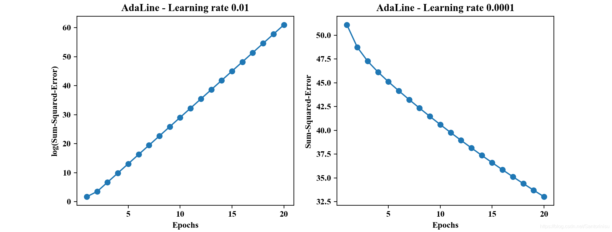
由上图可以得知,左图(left-figure)的收敛曲线是发散的,且由于随着迭代次数的增加,数值增大趋势明显,且取值范围较大,故对其进行对数缩放处理。这一点可以从“小球凹地滚动”方向进行理解,学习率过大,权重更新幅度显然容易超过稳定最优解。与此相,与学习率设定较小对应的右图(right-figure)逐步搜索到最优解,但是需要更多的迭代次数才可能趋于最优解。
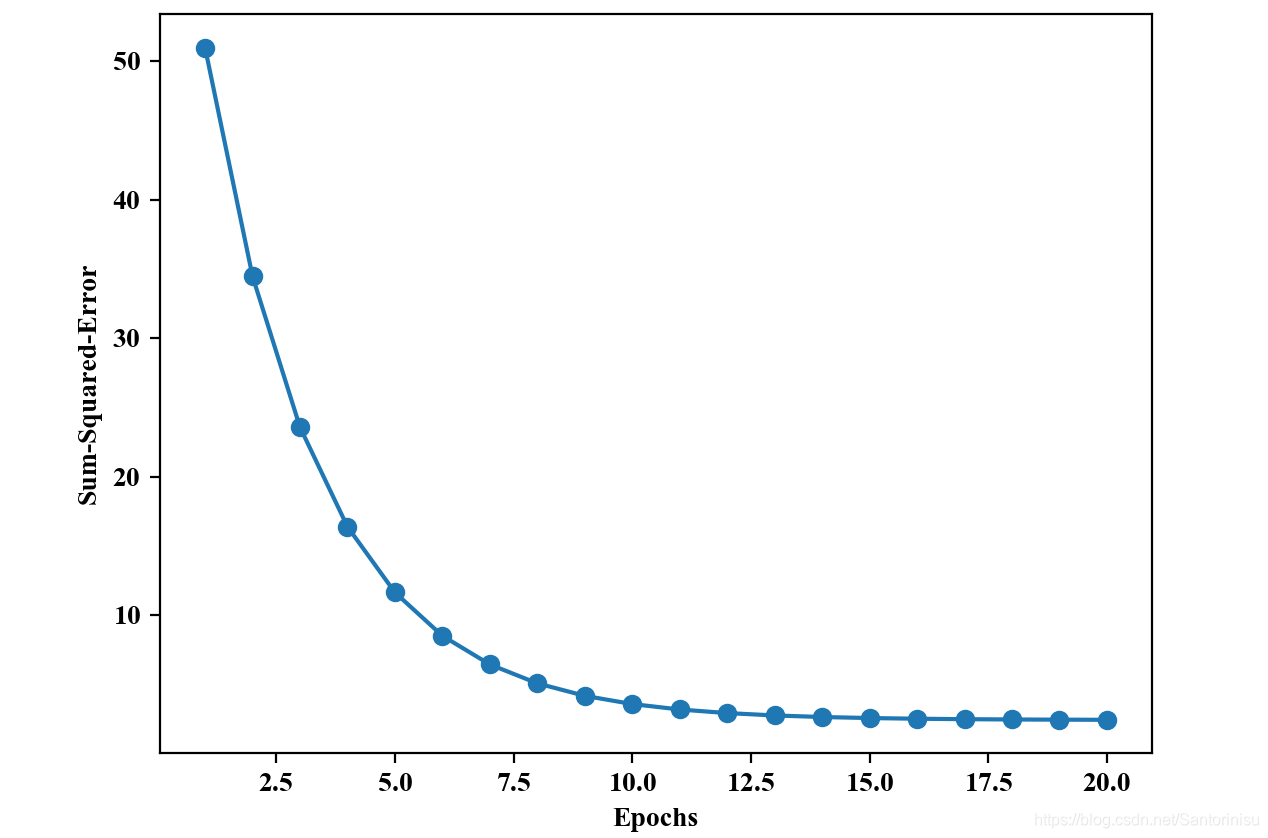
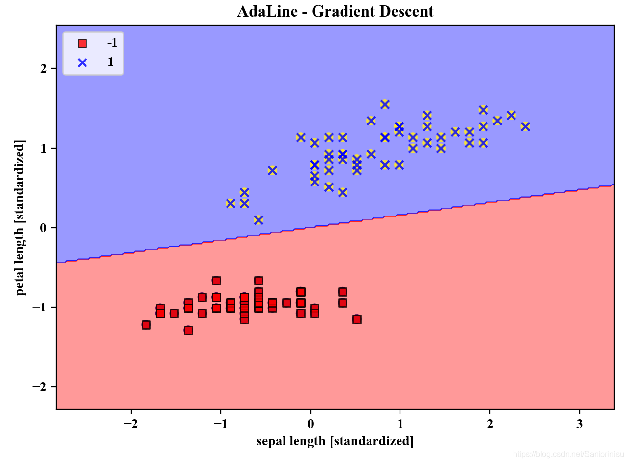
2、标准化模式下批处理AdaLine收敛曲线与划分边界
以下两图分别为进行标准化处理后,批处理AdaLine的收敛曲线和划分边界。其中,由第一幅子图可以得知,该算法针对标准化处理后的训练数据,收敛速度较快,训练效果较佳。
3、标准化模式下StochastisGD-Based AdaLine收敛性能与划分边界
以类似于标准化模式下进行批处理AdaLine的分析方式,此处也运行基于随机梯度下降方式的AdaLine算法于标准化后的训练数据集。相应地,收敛曲线和划分边界亦刻画至如下两幅子图。
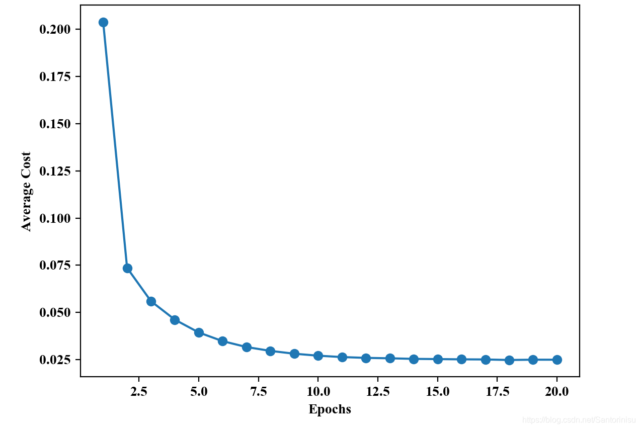
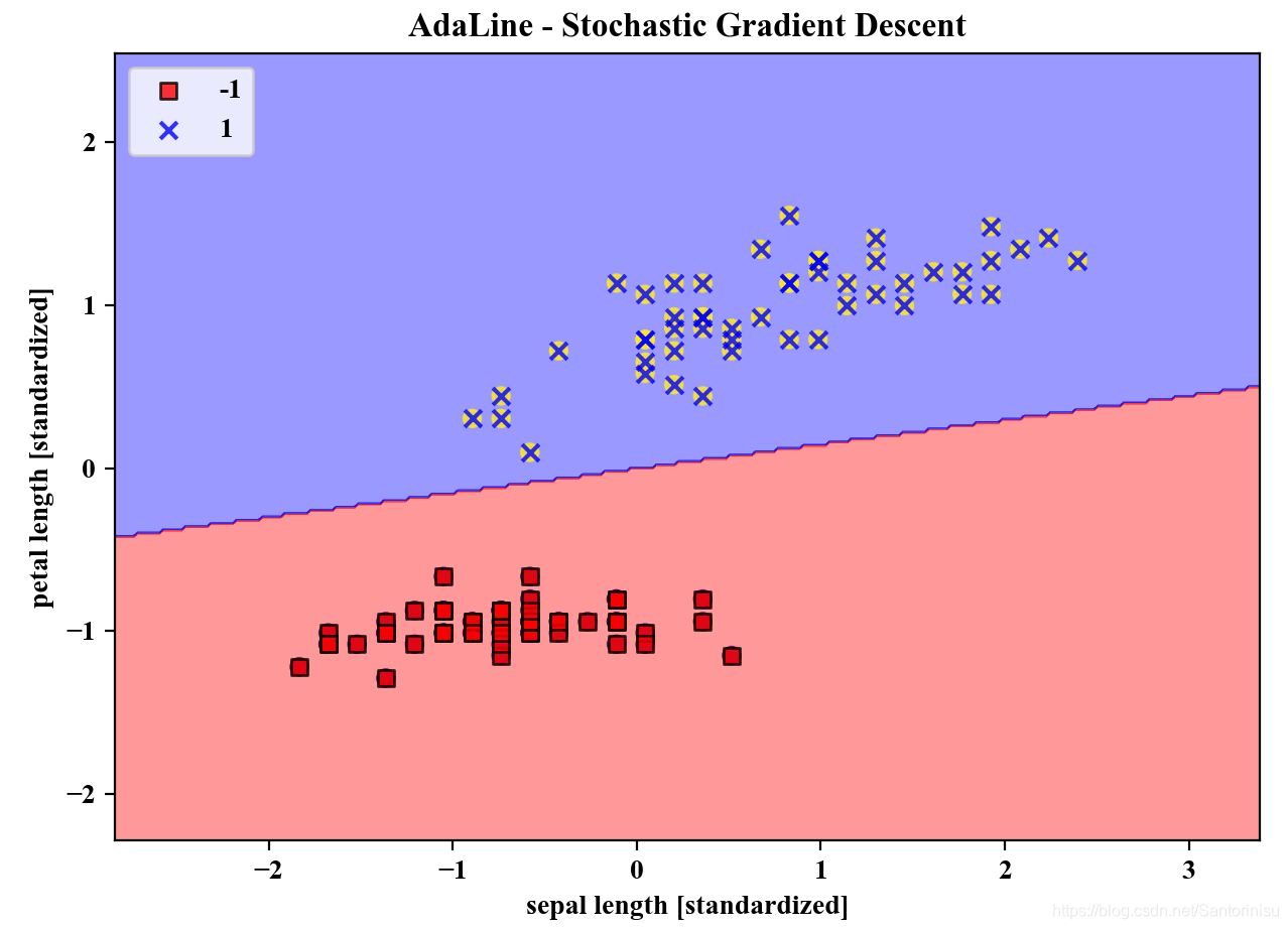
由收敛曲线子图可以得知,以随机梯度下降模式进行的AdaLine算法训练,收敛速度相对较快,原因在于相比批处理模式的权重更新,每条数据集更新依赖于上次迭代的整体效果,而后者权重的更新以递进方式更新,后一条训练数据集依赖于前一条的更新方向。由此可以得知数据集训练顺序的变化对训练效果的影响也是值得重点关注。
参考文献
Sebastian Raschka, Vahid Mirjalili. Python机器学习第二版. 南京:东南大学出版社,2018.


 432
432


 被折叠的 条评论
为什么被折叠?
被折叠的 条评论
为什么被折叠?
 到【灌水乐园】发言


