ML 14 part2 principal component analysis

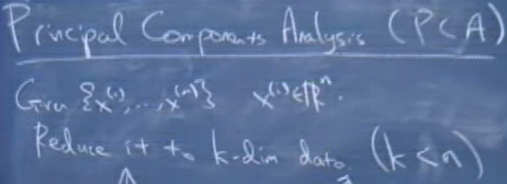
Given m samples in $R^n$

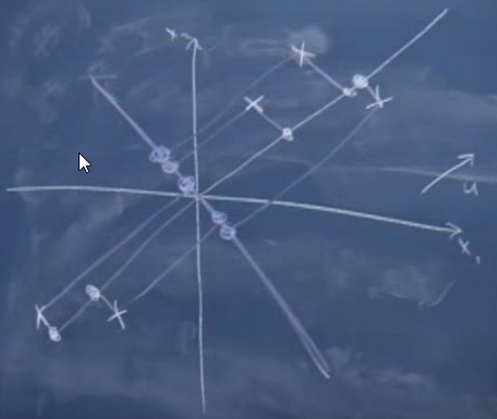
The goal is to find the direction $u$ along which maximizing the sum of projection of each point $u$


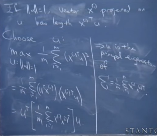
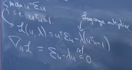
So to speak, $u$ ought to be the eigenvectors of the matrix $\Sigma$

Here we reduce n-dimension space down to k-dimension subspace which is composed of $u_1$, $u_2$, … ,$u_k$ basis

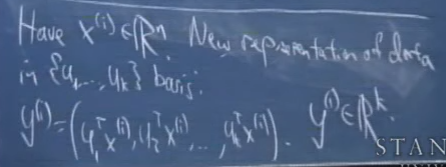
Given any x in n-dimension space, we can express it in k-dimension space as
$(u_1^Tx, u_2^Tx, \cdots, u_k^Tx)$. In other words, we project $x \in R^n$ into subspace $\{u_1, u_2, \cdots, u_k\} \in R^k$

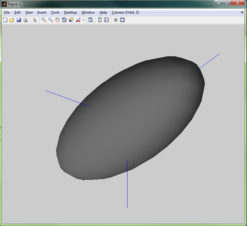
In order to perceive PCA algorithm more intuitive, we use matlab to draw some figures.

X0=read_obj('football1.obj'); % seahorse_extended.obj');
vertex=X0.xyz';  %坐标
faces=X0.tri'; %三角形顺序索引
center0 = mean(vertex,1);

% display the mesh
clf;
plot_mesh(vertex, faces);
shading interp;

[pc,scores,pcvars] = princomp(vertex);
u1 = pc(:,1);
u2 = pc(:,2);
u3 = pc(:,3);
% 
% 
hold on 
center = [];
center = [center ;center0];
center = [center ; center0 + u1'*20];
% center = [center ;center0];
% center = [center ; center0 + u1'*-20];
center = [center ;center0];
center = [center ; center0 + u2'*20];
% center = [center ;center0];
% center = [center ; center0 + u2'*-20];
center = [center ;center0];
center = [center ; center0 + u3'*20];
% center = [center ;center0];
% center = [center ; center0 + u3'*-20];
plot3 (center(:,1), center(:,2), center(:,3), '-*');

The core PCA algorithm is implemented in princomp function. the document of princomp says:

[COEFF,SCORE,latent,tsquare] = princomp(X)
COEFF = princomp(X) performs principal components analysis (PCA) on the n-by-p data matrix X, and returns the principal component coefficients, also known as loadings. Rows of X correspond to observations, columns to variables. COEFF is a p-by-p matrix, each column containing coefficients for one principal component. The columns are in order of decreasing component variance.
The scores are the data formed by transforming the original data into the space of the principal components. The values of the vector latent are the variance of the columns of SCORE. Hotelling’s T^2 is a measure of the multivariate distance of each observation from the center of the data set.

Expressing in our own language, the columns of COEFF is the eigenvectors of matrix $\Sigma$ which are the basis of the reduced space. In the document, principal components are their aliases.

In our case, because the dimension of original space is 3, the dimension of reduced space must be less than or equal to 3.
Then the data in original space can be reduced into the reduced space by means of dot product with each principal component to constitute a new point in reduced space.

the result picture seems like:

Due to the fact that I am fond of sharing, I would like to release the whole matlab source code:

complete MATLAB source code

Application in face recognition

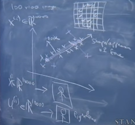
Assuming faces are encoded in 100*100 images, each image consists in 10000 pixels, which means each image $x \in R^{10000}$. Every pixel in the image stands for a dimension of the space.

Each image can be expressed a dot in $R^{10000}$, then we can solve the k top eigenvectors of $\Sigma$ in which each eigenvector can denote a people’s face.

say if we get a new face image, then we can project it on each eigenvector of subspace $R^k$. The large the projection is, more like these two faces are.