


数据集

import matplotlib.pyplot as plt
import numpy as np
from sklearn.metrics import classification_report
from sklearn import preprocessing
# 数据是否需要标准化,scale = True要做标准化,等于Flase不做标准化
scale = True
# 载入数据
data = np.genfromtxt("LR-testSet.csv", delimiter=",")
x_data = data[:,:-1]
y_data = data[:,-1]

def plot():
    x0 = []
    x1 = []
    y0 = []
    y1 = []
    # 切分不同类别的数据
    for i in range(len(x_data)):
        if y_data[i]==0:
            x0.append(x_data[i,0])
            y0.append(x_data[i,1])
            #(x0,y0)0类坐标
        else:
            x1.append(x_data[i,0])
            y1.append(x_data[i,1])
            #(x1,y1)1类坐标

    # 画图
    scatter0 = plt.scatter(x0, y0, c='b', marker='o')
    scatter1 = plt.scatter(x1, y1, c='r', marker='x')
    #画图例
    plt.legend(handles=[scatter0,scatter1],labels=['label0','label1'],loc='best')

plot()
plt.show()

# 数据处理,添加偏置项
x_data = data[:,:-1]
y_data = data[:,-1,np.newaxis]

print(np.mat(x_data).shape)
print(np.mat(y_data).shape)
# 给样本添加偏置项,加上100行1列的偏置项且里面都是数字都是1
X_data = np.concatenate((np.ones((100,1)),x_data),axis=1)
print(X_data.shape)

def sigmoid(x):
    return 1.0/(1+np.exp(-x))

def cost(xMat, yMat, ws):
    left = np.multiply(yMat, np.log(sigmoid(xMat*ws)))
    right = np.multiply(1 - yMat, np.log(1 - sigmoid(xMat*ws)))
    return np.sum(left + right) / -(len(xMat))

def gradAscent(xArr, yArr):

    if scale == True:
        xArr = preprocessing.scale(xArr)
    xMat = np.mat(xArr)
    yMat = np.mat(yArr)

    lr = 0.001  #学习率
    epochs = 10000  #迭代的周期
    costList = []  #用于保存cost的值
    # 计算数据行列数
    # 行代表数据个数,列代表权值个数
    m,n = np.shape(xMat)
    # 初始化权值,全设为1
    ws = np.mat(np.ones((n,1)))

    for i in range(epochs+1):
        # xMat和weights矩阵相乘
        h = sigmoid(xMat*ws)
        # 计算误差
        ws_grad = xMat.T*(h - yMat)/m
        ws = ws - lr*ws_grad

        if i % 50 == 0:
            costList.append(cost(xMat,yMat,ws))
    return ws,costList


mat矩阵,dot是矩阵相乘,mul是按位相乘

sigmoid函数是分式,也就是h函数
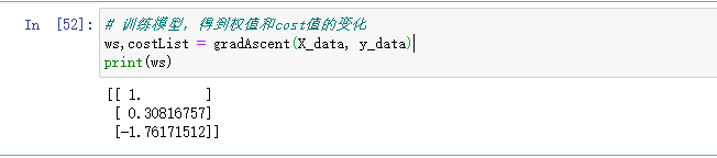
# 训练模型,得到权值和cost值的变化
ws,costList = gradAscent(X_data, y_data)
print(ws)
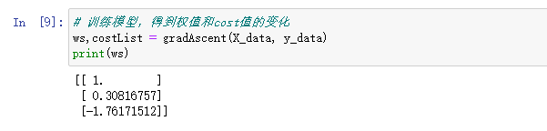
# 训练模型,得到权值和cost值的变化
ws,costList = gradAscent(X_data, y_data)
print(ws)
if scale == False:
    # 画图决策边界
    plot()
    x_test = [[-4],[3]]
    y_test = (-ws[0] - x_test*ws[1])/ws[2]
    plt.plot(x_test, y_test, 'k')
    plt.show()

# 画图 loss值的变化
x = np.linspace(0,10000,201)
plt.plot(x, costList, c='r')
plt.title('Train')
plt.xlabel('Epochs')
plt.ylabel('Cost')
plt.show()

# 预测
def predict(x_data, ws):
    if scale == True:
        x_data = preprocessing.scale(x_data)
    xMat = np.mat(x_data)
    ws = np.mat(ws)
    return [1 if x >= 0.5 else 0 for x in sigmoid(xMat*ws)]

predictions = predict(X_data, ws)

print(classification_report(y_data, predictions))

import matplotlib.pyplot as plt
import numpy as np
from sklearn.metrics import classification_report
from sklearn import preprocessing
from sklearn import linear_model
# 数据是否需要标准化
scale = False
# 载入数据
data = np.genfromtxt("LR-testSet.csv", delimiter=",")
x_data = data[:,:-1]
y_data = data[:,-1]

def plot():
    x0 = []
    x1 = []
    y0 = []
    y1 = []
    # 切分不同类别的数据
    for i in range(len(x_data)):
        if y_data[i]==0:
            x0.append(x_data[i,0])
            y0.append(x_data[i,1])
        else:
            x1.append(x_data[i,0])
            y1.append(x_data[i,1])

    # 画图
    scatter0 = plt.scatter(x0, y0, c='b', marker='o')
    scatter1 = plt.scatter(x1, y1, c='r', marker='x')
    #画图例
    plt.legend(handles=[scatter0,scatter1],labels=['label0','label1'],loc='best')

plot()
plt.show()

logistic = linear_model.LogisticRegression()
logistic.fit(x_data, y_data)
if scale == False:
    # 画图决策边界
    plot()
    x_test = np.array([[-4],[3]])
    y_test = (-logistic.intercept_ - x_test*logistic.coef_[0][0])/logistic.coef_[0][1]
    plt.plot(x_test, y_test, 'k')
    plt.show()

predictions = logistic.predict(x_data)

print(classification_report(y_data, predictions))


 1177
1177


 被折叠的 条评论
为什么被折叠?
被折叠的 条评论
为什么被折叠?
 到【灌水乐园】发言


