ColorFlow：基于检索增强的黑白漫画上色模型（包含论文代码详解）

Sherlock Ma

已于 2024-12-22 20:44:45 修改

阅读量1.2k

点赞数 22

分类专栏： AIGC 图像编辑 stable diffusion 文章标签：人工智能深度学习 AIGC AI作画

于 2024-12-22 20:44:04 首次发布

本文链接：https://blog.csdn.net/sherlockMa/article/details/144610912

版权

AIGC 同时被 3 个专栏收录

31 篇文章

订阅专栏

图像编辑

4 篇文章

订阅专栏

stable diffusion

3 篇文章

订阅专栏

1.简介

这篇文章介绍了一个名为ColorFlow的先进模型，它专门设计用于给黑白图像序列上色，同时精确保持人物和对象的身份特征。ColorFlow模型的意义在于它能够利用参考图像中的颜色信息，为漫画、动画制作和黑白电影着色等任务提供强大的技术支持。

这项技术的应用不仅能够提高内容创作的效率，还能够增强最终作品的艺术表现力和观众的沉浸感，为艺术产业带来创新和活力。通过这项工作，ColorFlow框架不仅提升了艺术作品的创作效率和质量，而且扩展了艺术创作的边界，为艺术产业的数字化转型和创新发展注入了新的活力。

项目主页：ColorFlow

在线演示：https://huggingface.co/spaces/TencentARC/ColorFlow

代码地址：https://github.com/TencentARC/ColorFlow

权重地址：https://huggingface.co/TencentARC/ColorFlow/tree/main

论文地址：https://arxiv.org/abs/2412.11815

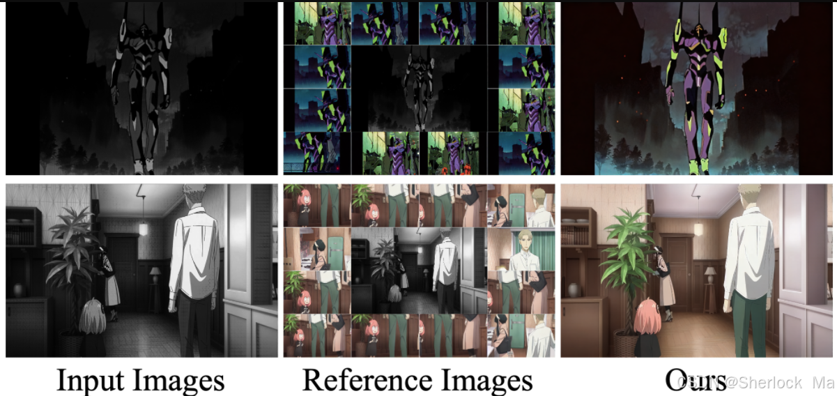
2.效果展示

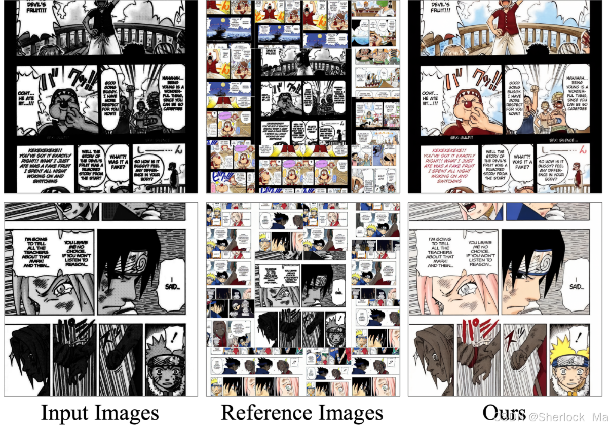
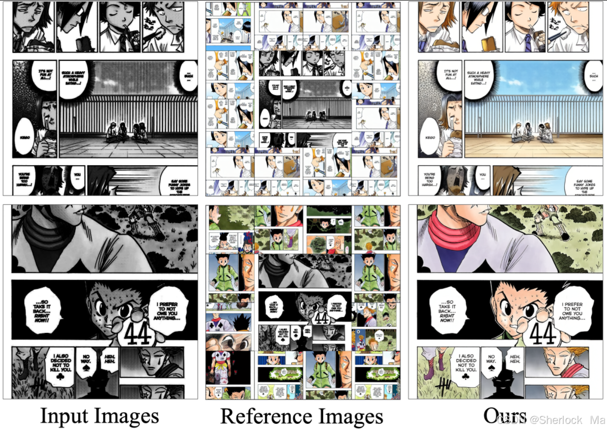
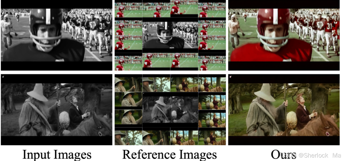
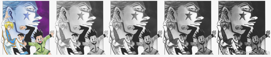
从左到右依次为：原图、和彩色参考图拼接的图、彩色输出图

3.论文解析

简介

最近，随着扩散模型带来前所未有的图像生成能力，人们对使用扩散模型进行上色的兴趣越来越大。然而，之前的大多数工作只考虑基本的文本到图像的范式，而没有参考颜色信息，这与实际应用相去甚远。虽然最近对AnimeDiffusion的研究已经探索了基于参考图像的动漫角色着色，但它仅支持对具有单一ID图像进行着色。

在这项工作中，作者引入了一个新的任务，基于参考的图像进行着色，其目的是将一系列的黑白图像转换为彩色图像。这一任务有很大的市场需求，但尚未解决。

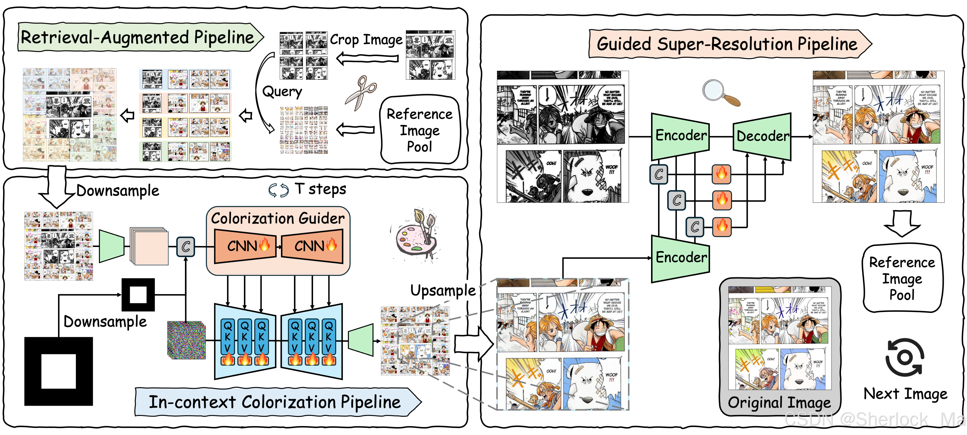
针对基于参考序列图像着色方法的不足，作者提出了一种适合工业应用的三阶段着色方法ColorFlow。分别是：

检索增强管道（RAP）：从参考图像池中提取相关的彩色图像块。
- 受检索增强生成（RAG）的启发，RAP在输入图像和参考池之间匹配ID相关的图像块，而无需对每个ID进行微调或进行显式ID embedding提取，使其更加方便。
上下文着色管道（ICP）：利用强大的上下文学习来准确检索颜色标识，并使用双分支设计执行着色。
- 着色模块核心部分采用两分支设计，分别实现图像颜色标识对应和着色。这种结构允许基础扩散模型的更深层更好地处理身份信息，同时保持其图像生成和着色能力。
- 利用扩散模型中的自注意机制，作者将参考图像和灰度图像放在同一画布上，使用一个复制权重的副本模型来提取它们的特征，并将这些特征逐层馈送到扩散模型中进行着色。
- 对于着色，我们使用低秩自适应（LoRA）来微调预训练的基础扩散模型，保留其着色功能。
引导超分辨率管道（GSRP）：上采样以生成高分辨率彩色图像。
- 作者还引入了引导超分辨率流水线，以减少彩色化过程中的结构细节失真。通过将高分辨率黑白白色漫画与低分辨率彩色输出集成，GSRP增强了细节恢复并提高了输出质量。

我们将在下文进行更详细的介绍。

作者构建了一个由30个漫画章节组成的数据集ColorFlow-Bench，每个章节包含50个白色漫画和40个参考图像。结果表明，ColorFlow在像素级和图像级评估中的五个指标上均实现了最先进的性能。

方法

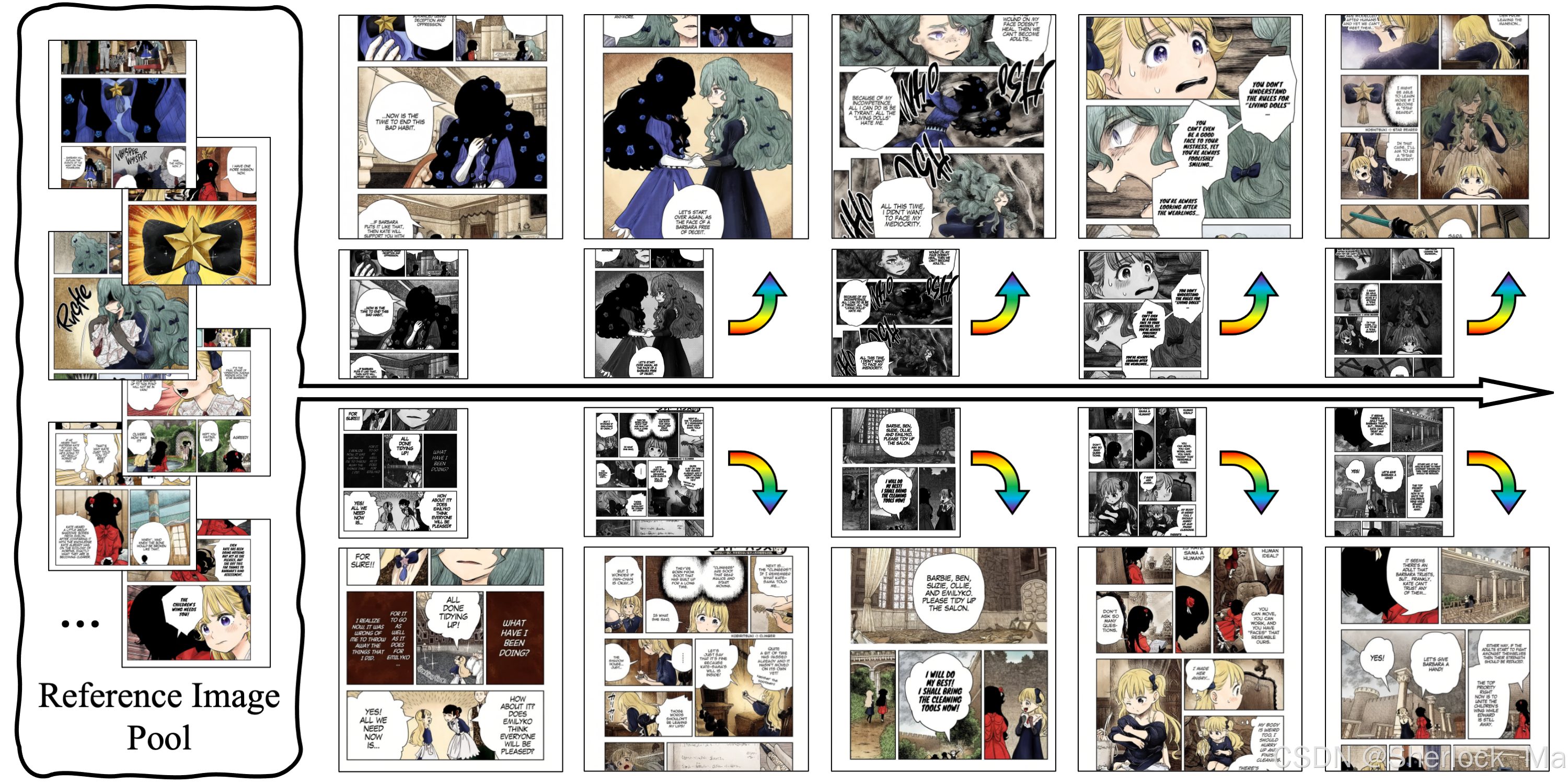
本工作的目标是使用彩色图像作为参考对黑白白色图像进行着色，确保整个图像序列中人物、对象和背景的一致性。如图所示，作者的框架由三个主要组件组成：检索增强管道，上下文着色管道和引导超分辨率管道。

检索增强管道

检索增强管道（RAP）旨在识别和提取相关的彩色参考图，以指导着色过程。

为了实现这一点，首先将输入的黑白图像分成四个重叠的块：左上、右上、左下和右下。每个块覆盖原始图像尺寸的四分之三，以确保保留重要细节。对于每个彩色参考图像，分别创建五个patch：相同的四个重叠patch和一张完整的图像，以提供一组全面的参考数据。
接下来，作者采用预训练的CLIP图像编码器来为输入图像的补丁生成图像嵌入Ebw，并为参考补丁生成Eref。这些嵌入定义如下： $E_{bw}=f_{CLIP}(P_{bw}) \: and \:E_{ref}=f_{CLIP}(P_{ref})$ ，其中Pbw表示黑白patch，Pref表示彩色参考patch。
对于每一个来自输入图像的四个patch，我们计算其嵌入与参考patch的嵌入之间的余弦相似度S： $S(a,b)=\frac{a\cdot b}{\left \| a \right \|\cdot \left \| b \right \|}$
我们为每个query patch定义前三个相似的patch如下： $Top_3(E^{(i)}_{bw})=\left \{ E^{(j_1)}_{ref},E^{(j_2)}_{ref},E^{(j_1)}_{ref}|j_k\in argmax_k S(E^{(i)}_{bw},E^{(k)}_{ref}),k=1,2,3\right \}$ ，对于i ∈ {0，1，2，3}，其中 $E^{(i)}_{bw}$ 表示第i个query patch的嵌入， $E^{(k)}_{ref}$ 表示对应的参考patch的嵌入。
在识别每个query区域的前三个相似patch后，我们将这些选定的patch拼接到黑白图像的左上角、右上角、左下角和右下角，以创建合成图像 $C_{bw}$ ，如图所示。这种空间布置确保了检索到的颜色信息的准确放置，增强了着色过程的上下文相关性。此外，我们通过类似地将对应于黑白图像块的原始彩色版本拼接在一起来构造（ $C_{color}$ ）。这与（ $C_{bw}$ ）形成数据对，用于随后的着色训练。 （ $C_{bw}$ 是输入， $C_{color}$ 是标签）

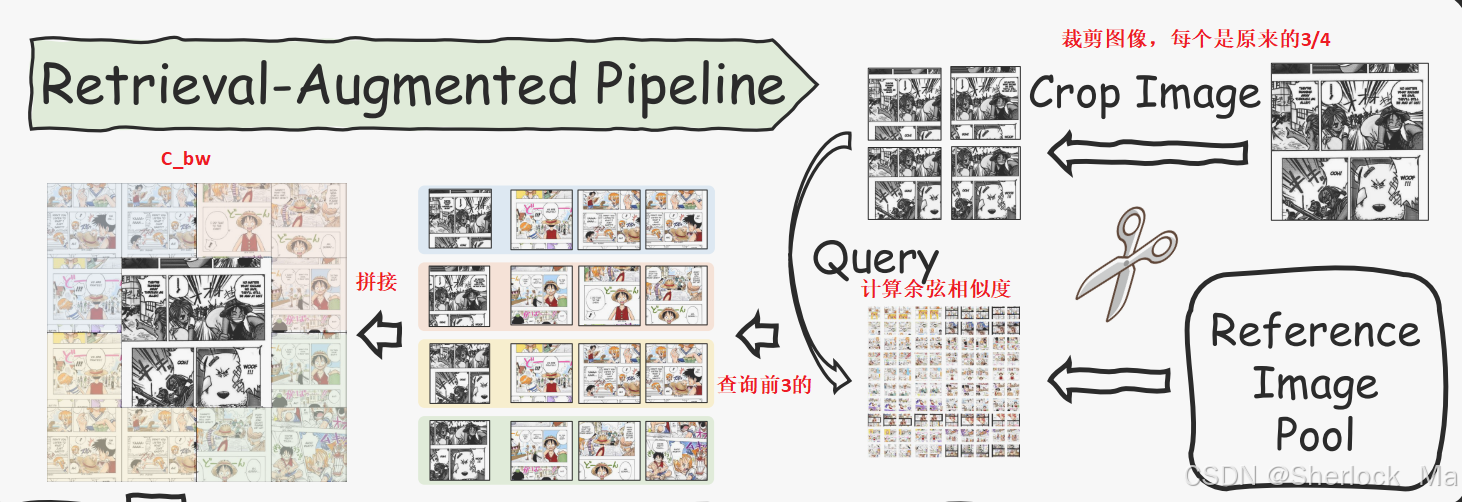
通过有效地收集最相关的上下文颜色信息，检索增强管道为该框架的下一阶段奠定了基础，确保生成的颜色与参考图像和谐一致。

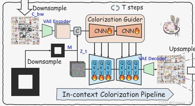
上下文着色管道

我们引入了一个称为着色引导器（Colorization Guider）的辅助分支，它有助于将条件信息纳入模型。该分支通过复制UNet中所有卷积层的权重来初始化。

着色引导器的输入包括噪声潜变量Zt、合成图像 $C_{bw}$ 经变分自动编码器处理后的输出 $VAE(C_{bw})$ 以及下采样后的掩码M。这些组成部分被连接起来，形成模型的综合输入。

来自着色引导器的特征将逐步集成到扩散模型的U-Net中，从而实现密集的逐像素条件嵌入。此外，我们利用轻量级LoRA（低秩自适应）方法来微调着色任务的扩散模型。

损失函数可以形式化如下： $L_{Color}=E_{t,C_bw,\epsilon _t}\left \| \epsilon _t-\epsilon _{\theta }(\left \{ VAE(C_{bw}),M,Z_t \right \} ,t)\right \|^2_2$ ，在训练期间，Zt通过前向扩散过程从VAE（ $C_{color}$ ）导出。该训练目标使模型能够有效地对输入潜在空间进行去噪，并在参考图像的指导下逐渐从黑白白色输入重建所需的彩色输出。

虽然我们没有显式地将彩色参考图像中的实例映射到黑白图像中的实例，但检索机制确保参考图像包含相似的内容。因此，模型自然地学习利用来自检索到的引用的上下文信息来准确地对黑白白色图像进行着色。

时间步移位采样。我们通过调整时间步长t′来修改采样策略： $t'=\frac{e^\mu }{e^\mu +(\frac{T}{t}-1)}T,\; \; \; t\sim \textup{u}(0,T]$ ，这个公式的目的是在生成过程中给予高时间步更高的权重，从而增强彩色化过程的效果。通过调整 µ 的值，可以控制高时间步在采样中的重要性。

在本工作中，作者将µ设置为1.5。这种调整使模型能够强调这些更高的时间步长，从而增强着色过程的有效性。

ScreenStyle样式增强：ScreenVAE可以将彩色漫画自动转换为日本黑白动漫风格。在这项工作中，作者通过在灰度图像和由ScreenVAE生成的输出之间执行随机线性插值来增强输入图像。

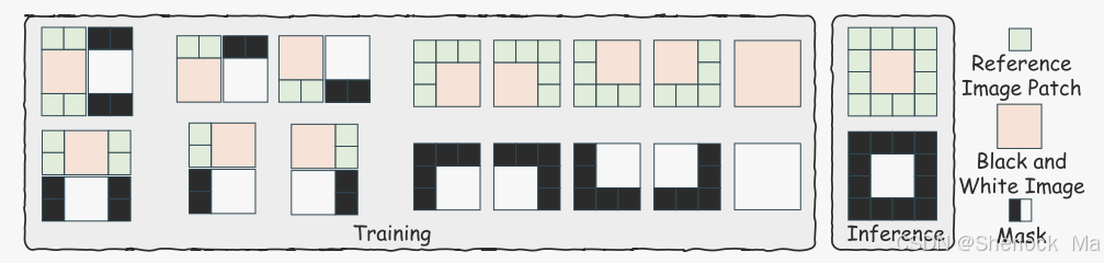
从左至右：彩色漫画，灰度漫画，灰度漫画和ScreenVAE输出之间的线性插值，比例为0.66和0.33，ScreenVAE输出。

Patch-Wise训练策略：为了解决高分辨率图像训练的大量计算需求，我们引入了一种分片训练策略。在训练过程中，我们从参考图像块中随机裁剪片段和对应掩码，确保始终包含整个黑白白色图像区域。

为了进一步提高性能，我们对输入图像进行了下采样，在保留关键细节的同时减少了计算负载。这种策略显著缩短了每次迭代的训练时间，促进了更快的模型收敛。

在推理过程中，我们使用完整的拼接图像来最大限度地提高着色的上下文信息的可用性。

（训练过程中使用不完整的拼接图训练，推理使用完整的进行推理）

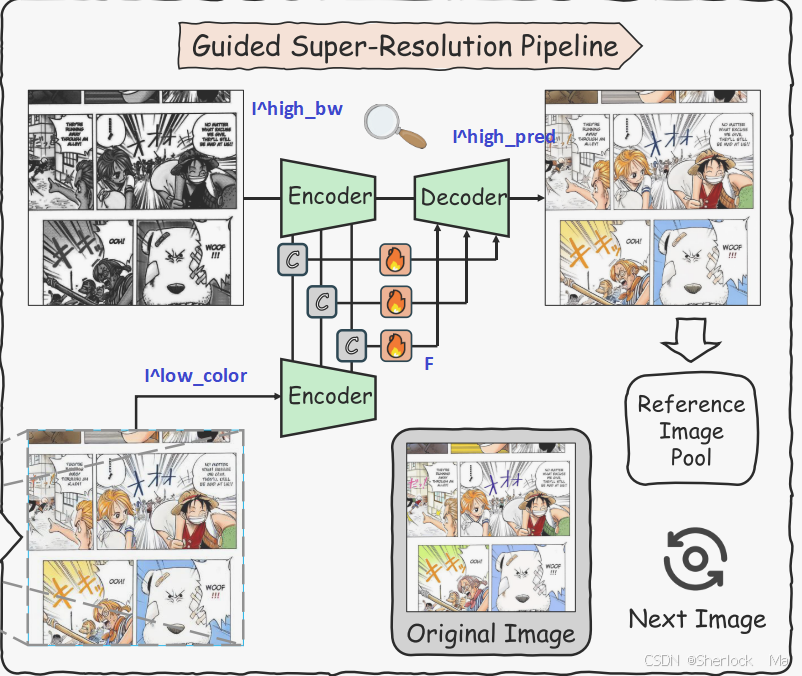
左侧框显示来自训练阶段的分段拼接图像，相应的掩码也相应地分段。右边的框表示完整的拼接图像和推理阶段的掩码。

引导超分辨率管道

引导超分辨率管道旨在解决着色期间的下采样相关的挑战，并减少在潜在解码器D的输出中经常看到的结构失真。这些问题会严重影响生成图像的质量。该流水线将高分辨率黑白图像 $I^{high}_{bw}$ 和由上下文内着色管道产生的低分辨率彩色输出 $I^{low}_{color}$ 作为输入。目标是产生高分辨率彩色图像 $I^{high}_{pred}$ 。

为了实现这一点，作者首先使用线性插值对低分辨率彩色图像 $I^{low}_{color}$ 进行上采样，以匹配 $I^{high}_{bw}$ 的分辨率。然后通过VAE编码器E处理二者。
为了实现有效的特征集成，作者在VAE的编码器和解码器之间建立跳级引导(skip guidance)。来自两个编码器的中间特征被拼接并传递到融合模块F，融合模块F将拼接的信息发送到解码器中的对应层。这种多尺度方法增强了细节恢复。

该过程的总损失函数定义为： $L_{SR}=E[\left | I^{high}_{bw} -D(F(concat(E_{features}(I^{high}_{bw}),E_{features}(Up_{sample}(I^{low}_{color})))))\right |_1]$ ，其中 $E_{features}$ 表示从VAE编码器提取的中间特征。该管道有效地解决了与下采样和结构失真相关的问题，从而获得更高质量的最终输出。

实验

数据集和基准测试

训练数据：在这项研究中，作者制作了迄今为止最大的漫画着色数据集，包括来自各种开放在线存储库的50000多个公开可用的彩色漫画章节序列，过滤掉黑白白色漫画后，产生了超过170万张图像。对于每个漫画帧，作者从相应的漫画章节中随机选择至少20个额外的帧来构建一个多样化的参考图像池。随后，作者利用CLIP图像编码器来识别和检索12个最相关的参考图像块。这种选择记录有助于后续训练，同时最大限度地减少冗余计算。

基准测试：为了评估作者提出的漫画着色框架的性能，作者建立了一个基准，包括30个漫画章节，不包括在训练阶段出现的数据。每一章都有40张参考图片和50页黑白漫画，并提供两种风格：screenstyle和灰度图像。作者使用以下几个指标来评估着色的质量和保真度：CLIP图像相似性（CLIP-IS），Fr 'echet起始距离（FID），峰值信噪比（PSNR），结构相似性指数（SSIM）和美学评分（AS）。这些指标对着色过程进行了全面而全面的评估，不仅评估了生成图像的美学质量，还评估了它们与原始内容的一致性。

实现细节

作者的着色模型基于stable diffusion v1.5。作者使用8个NVIDIA A100 GPU对我们的模型进行了150000步的训练。此外，引导超分辨率管道在相同的硬件配置和学习速率下进行了30000次迭代训练。

4.代码解析

环境安装

按照官网教程，直接从requirements.txt安装即可。

conda create -n colorflow python=3.8.5
conda activate colorflow
pip install -r requirements.txt

然后运行app.py即可，模型会自动下载权重

python app.py

使用教程

选择输入样式：灰度图(ScreenStyle)、线稿。
上传您的图像：使用“上传”按钮选择要上色的图像。
预处理图像：点击“预处理”（Preprocess (Decolorize)）按钮以去色图像。
上传参考图像：上传多张参考图像以指导上色。
设置采样参数（可选）：调整设置并点击上色（Colorize）按钮。

推理代码解析

extract_line_image()

这个函数用于调整图像尺寸，然后去色或提取线稿。

首先通过process_image()将图像尺寸调整为tar_width/tar_height的1.5倍
对于GrayImage(ScreenStyle)模式，执行去色操作：
1. 使用to_screen_image()转换为灰度图
2. 将原图和灰度图合并
对于Sketch模式，执行提取线稿操作

def extract_line_image(query_image_, input_style, resolution):      # 去色/提取线稿  query_image_:源图 input_style:输入类型(去色模式还是提取线稿) resolution:输出分辨率
    ...

    query_image = process_image(query_image_, int(tar_width*1.5), int(tar_height*1.5))  # 调整为目标尺寸
    if input_style == "GrayImage(ScreenStyle)":     # 去色
        extracted_line = to_screen_image(query_image)      # 转换为灰度图 
        extracted_line = Image.blend(extracted_line.convert('L').convert('RGB'), query_image.convert('L').convert('RGB'), 0.5)      # 将两个灰度图像按 50% 的透明度进行融合，生成最终的线稿图像
        input_context = extracted_line
    elif input_style == "Sketch":       # 线稿
        query_image = query_image.convert('L').convert('RGB')
        extracted_line = extract_lines(query_image)
        extracted_line = extracted_line.convert('L').convert('RGB')
        input_context = extracted_line
    torch.cuda.empty_cache()
    return input_context, extracted_line, input_context

process_image()

首先来看process_image()，由于将图像调整至目标尺寸（target_width/height，需要重要的是，这里是tra_width/height的1.5倍）具体步骤如下：

计算比例误差：根据输入图像和目标尺寸的比例，计算两者的比例误差。
判断是否直接缩放：如果比例误差小于0.15，则直接将图像缩放到目标尺寸；否则，先裁剪图像以匹配目标比例，再缩放到目标尺寸。
返回处理后的图像：最终返回转换为RGB格式的处理后图像。

def process_image(image, target_width=512, target_height = 512):
    img_width, img_height = image.size
    img_ratio = img_width / img_height
    
    target_ratio = target_width / target_height
    
    ratio_error = abs(img_ratio - target_ratio) / target_ratio
    
    if ratio_error < 0.15:      # 如果比例误差小于0.15，则直接将图像缩放到目标尺寸
        resized_image = image.resize((target_width, target_height), Image.BICUBIC)
    else:       # 否则，先裁剪图像以匹配目标比例，再缩放到目标尺寸。
        if img_ratio > target_ratio:
            new_width = int(img_height * target_ratio)
            left = int((0 + img_width - new_width)/2)
            top = 0
            right = left + new_width
            bottom = img_height
        else:
            new_height = int(img_width / target_ratio)
            left = 0
            top = int((0 + img_height - new_height)/2)
            right = img_width
            bottom = top + new_height
        
        cropped_image = image.crop((left, top, right, bottom))
        resized_image = cropped_image.resize((target_width, target_height), Image.BICUBIC)
    
    return resized_image.convert('RGB')     # 最终返回转换为RGB格式的处理后图像。

去色

接着我们看to_screen_image()

def to_screen_image(input_image):   # 转换为适合ScreenVAE模型处理的格式，并通过模型生成新的图像。
    global opt
    global ScreenModel
    input_image = input_image.convert('RGB')
    input_image = get_ScreenVAE_input(input_image, opt)
    h = input_image['h']
    w = input_image['w']        # tar_w
    ScreenModel.set_input(input_image)      # 设置模型输入：将预处理后的图像数据传递给ScreenModel模型。
    fake_B, fake_B2, SCR = ScreenModel.forward(AtoB=True)   # CycleGANSTFT 前向传播     [b,1,tar_w,tar_h]=[b,1,960,960]  SCR:[b,4,tar_w,tar_h]=[b,4,960,960]
    images=fake_B2[:,:,:h,:w]
    im = util.tensor2im(images)     # tensor转numpy
    image_pil = Image.fromarray(im)     # PIL
    torch.cuda.empty_cache()
    return image_pil

其中 get_ScreenVAE_input()如下，用于生成ScreenModel的输入数据：

def get_ScreenVAE_input(A_img, opt):

    L_img = A_img
    
    ...
    A_transform = get_transform(opt, transform_params, grayscale=False)     # Compose(Lambda()ToTensor()Normalize(mean=(0.5, 0.5, 0.5), std=(0.5, 0.5, 0.5)))
    L_transform = get_transform(opt, transform_params, grayscale=True)      # Compose(Grayscale(num_output_channels=1) Lambda() ToTensor() Normalize(mean=(0.5,), std=(0.5,)))
    A = A_transform(A_img)      # [3,原尺寸，原尺寸]
    L = L_transform(L_img)      # [1,原尺寸，原尺寸]
    
    tmp = A[0, ...] * 0.299 + A[1, ...] * 0.587 + A[2, ...] * 0.114     # RGB到灰度的转换公式
    Ai = tmp.unsqueeze(0)
    
    return {'A': A.unsqueeze(0), 'Ai': Ai.unsqueeze(0), 'L': L.unsqueeze(0), 'A_paths': '', 'h': oh, 'w': ow, 'B': torch.zeros(1),
                'Bs': torch.zeros(1),
                'Bi': torch.zeros(1),
                'Bl': torch.zeros(1),}

接着我们看如下代码：

extracted_line = Image.blend(extracted_line.convert('L').convert('RGB'), query_image.convert('L').convert('RGB'), 0.5)

extracted_line.convert('L'): 将名为extracted_line的图像转换为灰度图像（'L'模式）。如果extracted_line已经是灰度图像，则此步骤不会改变图像。
query_image.convert('L'): 将名为query_image的图像也转换为灰度图像。
.convert('RGB'): 将上述两个灰度图像转换回RGB模式。这一步是必要的，因为blend函数需要两个图像在相同的颜色模式下工作。
Image.blend(): 这是Pillow库中的一个函数，它用于将两个图像按照指定的alpha值进行混合。alpha值决定了第一个图像的透明度：alpha=1时完全透明，alpha=0时完全不透明。0.5意味着两个图像各占一半，即50%的透明度。

这行代码的作用是将extracted_line和query_image两个图像转换为灰度图，然后再转换回RGB模式，并以50%的透明度进行混合，生成一个新的图像。这个新的图像会是两个原始图像的线性混合结果。

提取线稿

其中extract_lines()的核心部分如下：

with torch.no_grad():           # 提取线稿
    y = line_model(tensor)

colorize_image()

该函数用于图像上色

1.预处理

导入掩码validation_mask
生成用于拼接黑白和彩色参考图的query_image_bw，尺寸为[tar_width,tar_height]
生成query_image_vae：用于超分时的输入
生成query_patches_pil：把原图切成四块含重复部分的块，尺寸是原图2/3，即[2/3*tar_width,2/3*tar_height]，位置分别是原来的四个角（可参照论文图片理解）
生成reference_patches_pil：生成参考图的裁切，一共5*ref_num张，
1. 比如输入3张参考图，这里就是15张，其中3张是原参考图，尺寸和目标输出尺寸一样；剩下12张的每块尺寸是原图2/3，位置分别是原来的四个角

# 1.预处理
validation_mask = Image.open('./assets/mask.png').convert('RGB').resize((tar_width*2, tar_height*2))    # 掩码图
gr.Info("Image retrieval in progress...")       #
query_image_bw = process_image(input_context, int(tar_width), int(tar_height))      # 用于后面拼接灰度图和彩色图
query_image = query_image_bw.convert('RGB')    # 转换为RGB，用于后面拼接灰度图和彩色图
query_image_vae = process_image(VAE_input, int(tar_width*1.5), int(tar_height*1.5))     # 用于后面作为超分模型输入
reference_images = [process_image(ref_image, tar_width, tar_height) for ref_image in reference_images]      # 调整参考图像尺寸
query_patches_pil = process_image_Q_varres(query_image, tar_width, tar_height)      # 切分图像，面积是原来的2/3，位置分别是原来的四个角
reference_patches_pil = []
for reference_image in reference_images:
    reference_patches_pil += process_image_ref_varres(reference_image, tar_width, tar_height)   # 5*ref_num（列如3张参考图，这里就是15张） 分别是完整图和四个角的图，四角图面积分别是原来的2/3
combined_image = None

2.拼接原图和参考图

计算查询图像和参考图像的嵌入向量：使用 image_processor 和 image_encoder 将查询图像和参考图像转换为嵌入向量query_embeddings，尺寸为[4b,1024]和reference_patches_pil_gray，尺寸为[15,1024]。
计算余弦相似度：计算查询图像嵌入向量与参考图像嵌入向量之间的余弦相似度，并排序得到前3个最相似的参考图像索引top_k_indices。
创建组合图像：
1. 创建一个空白的组合图像，并将查询图像query_image_bw粘贴到中心位置。
2. 根据相似度排序结果，将最相似的参考图像片段reference_patches_pil[ref_index]粘贴到组合图像的四个角

# 2.按照相似度查找最高的top3，然后拼接原图和参考图
with torch.no_grad():
    clip_img = image_processor(images=query_patches_pil, return_tensors="pt").pixel_values.to(image_encoder.device, dtype=image_encoder.dtype)      # [4b,3,224,224]
    query_embeddings = image_encoder(clip_img).image_embeds     # CLIP [4b,1024]
    reference_patches_pil_gray = [rimg.convert('RGB').convert('RGB') for rimg in reference_patches_pil]
    clip_img = image_processor(images=reference_patches_pil_gray, return_tensors="pt").pixel_values.to(image_encoder.device, dtype=image_encoder.dtype)     # [ref_nums*5,3,224,224]=[15,3,224,224]
    reference_embeddings = image_encoder(clip_img).image_embeds     # [ref_nums*5,1024]=[15,1024]
    cosine_similarities = F.cosine_similarity(query_embeddings.unsqueeze(1), reference_embeddings.unsqueeze(0), dim=-1)     # 计算四角和参考图之间的余弦相似度 [4b,ref_nums*5]=[4,15]
    sorted_indices = torch.argsort(cosine_similarities, descending=True, dim=1).tolist()        # 排序 得到尺寸[4b,ref_nums*5]=[4,15]的列表，里面的值是索引
    top_k = 3
    top_k_indices = [cur_sortlist[:top_k] for cur_sortlist in sorted_indices]       # 得到尺寸[4b,3]=[4,3]的列表，里面的值是索引
    combined_image = Image.new('RGB', (tar_width * 2, tar_height * 2), 'white')     # 创建一个空白的组合图像
    combined_image.paste(query_image_bw.resize((tar_width, tar_height)), (tar_width//2, tar_height//2))     # 将查询图像（要上色的黑白图像）粘贴到中心位置。
    idx_table = {0:[(1,0), (0,1), (0,0)], 1:[(1,3), (0,2),(0,3)], 2:[(2,0),(3,1), (3,0)], 3:[(2,3), (3,2),(3,3)]}
    for i in range(2):      # 将最相似的参考图像片段粘贴到组合图像的四个角
        for j in range(2):
            idx_list = idx_table[i * 2 + j]
            for k in range(top_k):
                ref_index = top_k_indices[i * 2 + j][k]
                idx_y = idx_list[k][0]
                idx_x = idx_list[k][1]
                combined_image.paste(reference_patches_pil[ref_index].resize((tar_width//2-2, tar_height//2-2)), (tar_width//2 * idx_x + 1, tar_height//2 * idx_y + 1))

3.模型推理

# 3.模型推理
gr.Info("Model inference in progress...")
generator = torch.Generator(device='cuda').manual_seed(seed)
image = pipeline(       # [2*tar_width,2*tar_height]
    "manga", cond_image=combined_image, cond_mask=validation_mask, num_inference_steps=num_inference_steps, generator=generator
).images[0]

其中pipeline是 ColorFlowSDPipeline 类的 __call__ 方法，位于diffusers/pipelines/colorflow/pipeline_colorflow_sd.py，用于生成图像。主要步骤包括：

参数处理：检查并处理输入参数。(代码注释1-2)
编码提示：将文本提示编码为嵌入向量。(代码注释3)
1. 文本提示编码为嵌入向量的输入是'manga'，更多的起到的是占位作用。也会输入Unet进行推理
准备图像：根据配置调整输入图像和掩码。(代码注释4)
准备时间步：设置推理步骤和时间步。(代码注释5)
准备潜在变量：初始化潜在变量和条件潜在变量。(代码注释6-7)
去噪循环：通过多次迭代逐步生成图像。(代码注释8)
后处理：解码潜在变量为图像，并进行安全检查。

其中代码注释1-3的部分不多介绍。

准备图像

准备图像部分(代码注释4)的主要目的是生成三张图像，分别是

image，即image_A：将中心的黑白图像遮住，只保留彩色图像
image_bw，即image_B：将彩色图像遮住，只保留中心的黑白图像
掩码：中间白，四周黑

elif colorguider.config.conditioning_channels==9:
    width, height = image.size      # 2*tar_width,2*tar_height=1280

    center_width = width // 2       # tar_width=640
    center_height = height // 2
    crop_width = width // 2         # tar_width
    crop_height = height // 2

    left = (width - crop_width) // 2    # 320 中心图的起始坐标
    top = (height - crop_height) // 2
    right = left + crop_width       # 320 中心图的终止坐标
    bottom = top + crop_height  
    # 创建一个新的图像，大小与原图相同，填充为黑色
    image_A = Image.new('RGB', (width, height), (0, 0, 0))

    # 将原图粘贴到新图像的外围区域
    image_A.paste(image, (0, 0))

    # 将中心区域设置为黑色
    image_A.paste(Image.new('RGB', (crop_width, crop_height), (0, 0, 0)), (left, top))
    # 创建一个新的图像，大小与原图相同，填充为黑色
    image_B = Image.new('RGB', (width, height), (0, 0, 0))

    # 将原图的中心区域粘贴到新图像的中心区域

    image_B.paste(image.crop((left, top, right, bottom)), (left, top))

    image = self.prepare_image(     # 裁切，转tensor等一系列操作  [2b,3,2*tar_width,2*tar_height]=[2b,3,1280,1280]
        image=image_A,
        width=width,
        height=height,
        batch_size=batch_size * num_images_per_prompt,
        num_images_per_prompt=num_images_per_prompt,
        device=device,
        dtype=colorguider.dtype,
        do_classifier_free_guidance=self.do_classifier_free_guidance,
        guess_mode=guess_mode,
    )
    image_bw = self.prepare_image(
        image=image_B,
        width=width,
        height=height,
        batch_size=batch_size * num_images_per_prompt,
        num_images_per_prompt=num_images_per_prompt,
        device=device,
        dtype=colorguider.dtype,
        do_classifier_free_guidance=self.do_classifier_free_guidance,
        guess_mode=guess_mode,
    )

original_mask = transforms.ToTensor()(mask).to(device=device, dtype=image.dtype).unsqueeze(0)
# print(original_mask.shape)
original_mask=(1 - original_mask[:,0:1,:,:]).to(image.dtype)    # [b,1,2*tar_width,2*tar_height]

original_mask = torch.cat([original_mask] * 2)      # [2b,1,2*tar_width,2*tar_height]
height, width = image.shape[-2:]

image/image_A：

image_bw/image_B：

时间步（代码注释5）也不多介绍

准备潜在变量

准备潜在变量：生成潜在变量 latents 和噪声 noise。
准备条件潜在变量：
1. 使用 VAE 编码器对彩色参考图像进行编码，生成条件潜在变量 conditioning_latents。尺寸为[2b,4,160,160]（这个生成过程是DiagonalGaussianDistribution的sample()，参考图像超清化的encoder）
2. 对黑白图像进行编码，并生成相应的条件潜在变量 conditioning_latents_bw。尺寸为[2b,4,160,160]
3. 对原始掩码进行插值处理，以匹配条件潜在变量的尺寸。尺寸为[2b,1,160,160]
则将彩色、黑白和掩码的潜在信息拼接在一起。尺寸为[2b,9,160,160]

# 6. Prepare latent variables
num_channels_latents = self.unet.config.in_channels
latents, noise = self.prepare_latents(
    batch_size * num_images_per_prompt,
    num_channels_latents,
    height,
    width,
    prompt_embeds.dtype,
    device,
    generator,
    latents,
)

# 6.1 prepare condition latents
conditioning_latents=self.vae.encode(image).latent_dist.sample() * self.vae.config.scaling_factor   # [2b,4,160,160]
if colorguider.config.conditioning_channels==9:
    conditioning_latents_bw=self.vae.encode(image_bw).latent_dist.sample() * self.vae.config.scaling_factor
mask = torch.nn.functional.interpolate(     # [2b,1,160,160]
            original_mask, 
            size=(
                conditioning_latents.shape[-2], 
                conditioning_latents.shape[-1]
            ),
            mode='bilinear'
        )
# transforms.ToPILImage()((mask[0,:,:,:])).save(f"{device}_masks.png")
if colorguider.config.conditioning_channels==9:     # 将黑白、彩色、掩码的潜在信息拼起来 [2b,9,160,160]
    conditioning_latents = torch.concat([conditioning_latents, mask, conditioning_latents_bw],1)

其中prepare_latents()如下

def prepare_latents(self, batch_size, num_channels_latents, height, width, dtype, device, generator, latents=None):
    if latents is None:
            noise = randn_tensor(shape, generator=generator, device=device, dtype=dtype)

    latents = noise * self.scheduler.init_noise_sigma

生成colorguider_keep，用于colorguider的conditioning_scale

# 7.2 Create tensor stating which colorguiders to keep
colorguider_keep = []       # colorguider的conditioning_scale
for i in range(len(timesteps)):
    keeps = [
        1.0 - float(i / len(timesteps) < s or (i + 1) / len(timesteps) > e)
        for s, e in zip(control_guidance_start, control_guidance_end)
    ]
    colorguider_keep.append(keeps[0] if (isinstance(colorguider, ColorGuiderSDModel)) else keeps)

其值为

[1.0, 1.0, 1.0, 1.0, 1.0, 1.0, 1.0, 1.0, 1.0, 1.0]

去噪循环

# 8. Denoising loop
num_warmup_steps = len(timesteps) - num_inference_steps * self.scheduler.order

with self.progress_bar(total=num_inference_steps) as progress_bar:
    for i, t in enumerate(timesteps):
        # expand the latents if we are doing classifier free guidance
        latent_model_input = torch.cat([latents] * 2) if self.do_classifier_free_guidance else latents
        latent_model_input = self.scheduler.scale_model_input(latent_model_input, t)

        if guess_mode and self.do_classifier_free_guidance:
            ...
        else:
            control_model_input = latent_model_input
            colorguider_prompt_embeds = prompt_embeds

        if isinstance(colorguider_keep[i], list):
            ...
        else:
            colorguider_cond_scale = colorguider_conditioning_scale
            cond_scale = colorguider_cond_scale * colorguider_keep[i]

        # colorguider
        down_block_res_samples, mid_block_res_sample, up_block_res_samples = self.colorguider(      # colorguider
            control_model_input,        # 噪声z_t  [2b,4,160,160]
            t,
            encoder_hidden_states=colorguider_prompt_embeds,
            colorguider_cond=conditioning_latents,      # 彩色参考图+掩码+黑白参考图 [2b,9,160,160]
            conditioning_scale=cond_scale,
            guess_mode=guess_mode,
            return_dict=False,
        )
        
        # UNet预测噪声
        noise_pred = self.unet(
            latent_model_input,     # 噪声z_t  [2b,4,160,160]
            t,
            encoder_hidden_states=prompt_embeds,
            timestep_cond=timestep_cond,
            cross_attention_kwargs=self.cross_attention_kwargs,
            down_block_add_samples=down_block_res_samples,      # colorguider的下采样层
            mid_block_add_sample=mid_block_res_sample,
            up_block_add_samples=up_block_res_samples,
            added_cond_kwargs=added_cond_kwargs,
            return_dict=False,
        )[0]

        # perform guidance    
        if self.do_classifier_free_guidance:
            noise_pred_uncond, noise_pred_text = noise_pred.chunk(2)
            noise_pred = noise_pred_uncond + self.guidance_scale * (noise_pred_text - noise_pred_uncond)

        # 去噪 compute the previous noisy sample x_t -> x_t-1
        latents = self.scheduler.step(noise_pred, t, latents, **extra_step_kwargs, return_dict=False)[0]

        ...

if not output_type == "latent":
    image = self.vae.decode(latents / self.vae.config.scaling_factor, return_dict=False, generator=generator)[
        0
    ]
    image, has_nsfw_concept = self.run_safety_checker(image, device, prompt_embeds.dtype)
else:
    image = latents
    has_nsfw_concept = None

image = self.image_processor.postprocess(image, output_type=output_type, do_denormalize=do_denormalize)

colorguider

其中colorguider的流程如下：

预处理：将噪声和彩色、黑白、掩码拼接起来
输入分别经过Unet和paintingNet的下采样层
分别经过Unet和paintingNet的中间层
分别经过Unet（注意有来自Unet下采样层的跳级连接）和paintingNet的上采样层
返回paintingNet的下采样层、中间层、上采样层的隐藏层状态

预处理：将噪声和彩色、黑白、掩码拼接起来 [2b,4,160,160]+[2b,9,160,160]=[2,13,160,160]

# 2. pre-process
brushnet_cond=torch.concat([sample,brushnet_cond],1)    # 将噪声和彩色、黑白、掩码拼接起来 [2b,4,160,160]+[2b,9,160,160]=[2,13,160,160]
sample = self.conv_in_condition(brushnet_cond)      # 13->320

下采样

包括两个部分：Unet的下采样和paintingNet（具体是brushNet）的下采样

# 3. down
down_block_res_samples = (sample,)
for downsample_block in self.down_blocks:
    if hasattr(downsample_block, "has_cross_attention") and downsample_block.has_cross_attention:
        sample, res_samples = downsample_block(
            hidden_states=sample,
            temb=emb,
            encoder_hidden_states=encoder_hidden_states,
            attention_mask=attention_mask,
            cross_attention_kwargs=cross_attention_kwargs,
        )

    down_block_res_samples += res_samples

# 4. PaintingNet down blocks
brushnet_down_block_res_samples = ()
for down_block_res_sample, brushnet_down_block in zip(down_block_res_samples, self.brushnet_down_blocks):
    down_block_res_sample = brushnet_down_block(down_block_res_sample)
    brushnet_down_block_res_samples = brushnet_down_block_res_samples + (down_block_res_sample,)

其中除了最后一个外的downsample_block包括以下部分：

resnet块
交叉注意力，图像提供Q，文本通过KV

最后一个仅有用于下采样的resnet

hidden_states = resnet(hidden_states, temb, scale=lora_scale)
hidden_states = attn(
    hidden_states,
    encoder_hidden_states=encoder_hidden_states,
    cross_attention_kwargs=cross_attention_kwargs,
    attention_mask=attention_mask,
    encoder_attention_mask=encoder_attention_mask,
    return_dict=False,
)[0]

其中PaintingNet的下采样块brushnet_down_block的结构如下：

ModuleList(
  (0-3): 4 x Conv2d(320, 320, kernel_size=(1, 1), stride=(1, 1))
  (4-6): 3 x Conv2d(640, 640, kernel_size=(1, 1), stride=(1, 1))
  (7-11): 5 x Conv2d(1280, 1280, kernel_size=(1, 1), stride=(1, 1))
)

中间层

# 5. mid
if self.mid_block is not None:
    if hasattr(self.mid_block, "has_cross_attention") and self.mid_block.has_cross_attention:
        sample = self.mid_block(
            sample,
            emb,
            encoder_hidden_states=encoder_hidden_states,
            attention_mask=attention_mask,
            cross_attention_kwargs=cross_attention_kwargs,
        )
    else:
        sample = self.mid_block(sample, emb)

# 6. BrushNet mid blocks
brushnet_mid_block_res_sample = self.brushnet_mid_block(sample)

结构和上采样部分的类似，故不多展示

上采样

还是和之前一样，Unet的上采样和paintingNet的上采样分别处理

# 7. up
up_block_res_samples = ()
for i, upsample_block in enumerate(self.up_blocks):
    is_final_block = i == len(self.up_blocks) - 1

    res_samples = down_block_res_samples[-len(upsample_block.resnets) :]
    down_block_res_samples = down_block_res_samples[: -len(upsample_block.resnets)]

    # if we have not reached the final block and need to forward the
    # upsample size, we do it here
    if not is_final_block:
        upsample_size = down_block_res_samples[-1].shape[2:]

    if hasattr(upsample_block, "has_cross_attention") and upsample_block.has_cross_attention:
        sample, up_res_samples = upsample_block(
            hidden_states=sample,
            temb=emb,
            res_hidden_states_tuple=res_samples,
            encoder_hidden_states=encoder_hidden_states,
            cross_attention_kwargs=cross_attention_kwargs,
            upsample_size=upsample_size,
            attention_mask=attention_mask,
            return_res_samples=True
        )
    else:
        sample, up_res_samples = upsample_block(
            hidden_states=sample,
            temb=emb,
            res_hidden_states_tuple=res_samples,
            upsample_size=upsample_size,
            return_res_samples=True
        )

    up_block_res_samples += up_res_samples

# 8. BrushNet up blocks
brushnet_up_block_res_samples = ()
for up_block_res_sample, brushnet_up_block in zip(up_block_res_samples, self.brushnet_up_blocks):
    up_block_res_sample = brushnet_up_block(up_block_res_sample)
    brushnet_up_block_res_samples = brushnet_up_block_res_samples + (up_block_res_sample,)

其中，在Unet中，作者先使用concat将下采样的结果和中间层输出hidden_states拼在一起，然后使用resnet降回正常维度，再进行运算。

scaling

返回paintingNet的下采样层、中间层、上采样层的隐藏层状态

# 6. scaling
if guess_mode and not self.config.global_pool_conditions:
    ...
else:
    brushnet_down_block_res_samples = [sample * conditioning_scale for sample in brushnet_down_block_res_samples]    # conditioning_scale默认为1
    brushnet_mid_block_res_sample = brushnet_mid_block_res_sample * conditioning_scale
    brushnet_up_block_res_samples = [sample * conditioning_scale for sample in brushnet_up_block_res_samples]

...

if not return_dict:
    return (brushnet_down_block_res_samples, brushnet_mid_block_res_sample, brushnet_up_block_res_samples)

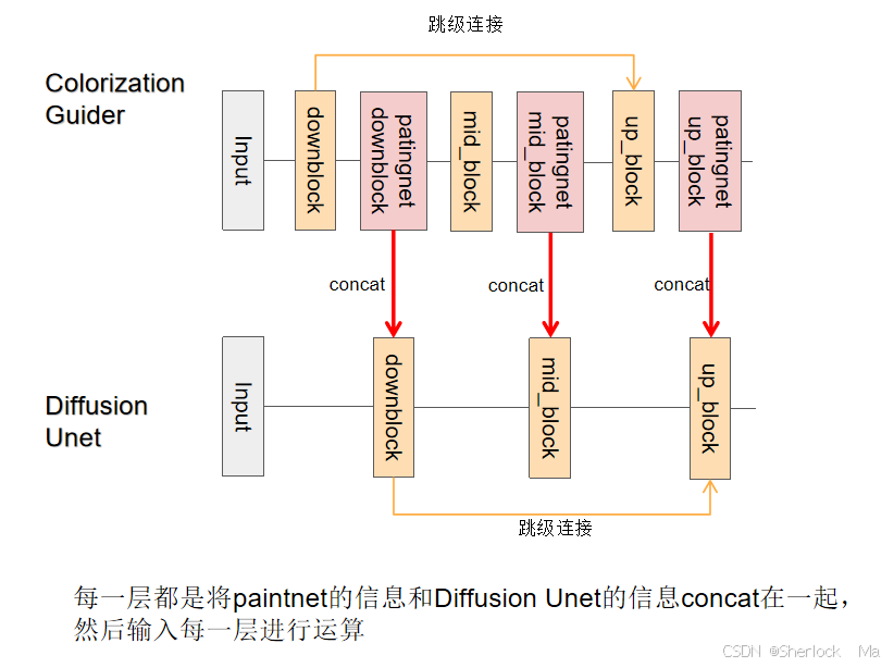
Unet

Unet的整体结构就不多介绍了，这里我们需要注意一点，在输入Unet的每一层之前，都会把来自paintingNet对应层的信息加上，然后再输入每一层进行处理。（见上图）

hidden_states = hidden_states + down_block_add_samples.pop(0)

4.图像超清化

# 4.图像超清化
gr.Info("Post-processing image...")
with torch.no_grad():
    width, height = image.size
    new_width = width // 2
    new_height = height // 2
    left = (width - new_width) // 2
    top = (height - new_height) // 2
    right = left + new_width
    bottom = top + new_height

    center_crop = image.crop((left, top, right, bottom))    # 把中间的生成的彩图剪出来  [tar_width,tar_height]
    up_img = center_crop.resize(query_image_vae.size)       # 放大到[1.5*tar_width,1.5*tar_height]
    test_low_color = transform(up_img).unsqueeze(0).to('cuda', dtype=weight_dtype)      
    query_image_vae = transform(query_image_vae).unsqueeze(0).to('cuda', dtype=weight_dtype)

    # 超分的两个Encoder
    h_color, hidden_list_color = pipeline.vae._encode(test_low_color,return_dict = False, hidden_flag = True)       # 将低分辨率彩色图编码，获取隐含特征。
    h_bw, hidden_list_bw = pipeline.vae._encode(query_image_vae, return_dict = False, hidden_flag = True)           # 将低分辨率黑白图编码，获取隐含特征。

    # 将两个Encoder的结果拼起来
    hidden_list_double = [torch.cat((hidden_list_color[hidden_idx], hidden_list_bw[hidden_idx]), dim = 1) for hidden_idx in range(len(hidden_list_color))]  # 在c维度进行特征融合

    # 将Encoder的特征进行处理
    hidden_list = MultiResNetModel(hidden_list_double)      # 使用多分辨率网络对拼接后的特征进行处理，生成新的隐含特征。

    # 超分Decoder
    output = pipeline.vae._decode(h_color.sample(),return_dict = False, hidden_list = hidden_list)[0]   # 解码生成最终的高分辨率彩色图像。
    # 归一化处理。
    output[output > 1] = 1      
    output[output < -1] = -1
    high_res_image = Image.fromarray(((output[0] * 0.5 + 0.5).permute(1, 2, 0).detach().cpu().numpy() * 255).astype(np.uint8)).convert("RGB")
gr.Info("Colorization complete!")
torch.cuda.empty_cache()
return high_res_image, up_img, image, query_image_bw    # 返回超分后的彩色图像，扩散生成的彩色图像，彩图和黑白图的拼接图和原始黑白图像

这段代码定义了一个图像预处理的转换管道 transform，用于将输入图像转换为适合神经网络模型训练的格式。具体功能如下：

ToTensor：将PIL图像或numpy数组转换为PyTorch张量，并将像素值从[0, 255]缩放到[0, 1]。
Normalize：对每个通道进行标准化处理，使用均值 [0.5, 0.5, 0.5] 和标准差 [0.5, 0.5, 0.5]，将数据分布调整到均值为0，标准差为1。

transform = transforms.Compose([
    transforms.ToTensor(),  
    transforms.Normalize(mean=[0.5, 0.5, 0.5], std=[0.5, 0.5, 0.5])  
])

encoder

其中vae._encode()如下：

首先通过encoder()编码，返回编码结果 h 和每一层的隐藏状态列表 hidden_list。
然后对编码结果 h 进行量化处理。在这里，self.quant_conv 是一个卷积层，它的目的是将输入 h 转换成一组“矩”（moments），这些矩通常是指概率分布的参数。在许多情况下，这些矩可能代表高斯分布的均值和方差。
使用上一步得到的矩 moments 来创建一个对角高斯分布（也称为正态分布）。DiagonalGaussianDistribution 是一个表示概率分布的类，它接受分布的参数（即矩）作为输入。在对角高斯分布中，每个维度（例如，每个像素位置）的分布是独立的，并且由其自己的均值和方差参数化。

class AutoencoderKL(ModelMixin, ConfigMixin, FromOriginalModelMixin):
    def _encode(
        self, x: torch.FloatTensor, return_dict: bool = True, hidden_flag = False
    ) -> Union[AutoencoderKLOutput, Tuple[DiagonalGaussianDistribution]]:
        if hidden_flag:
            h,hidden_list = self.encoder(x, hidden_flag = hidden_flag)      # 返回编码结果 h 和隐藏状态列表 hidden_list。
        else:
            h = self.encoder(x, hidden_flag = hidden_flag)

        moments = self.quant_conv(h)        # 对编码结果 h 进行量化处理，得到 moments。
        posterior = DiagonalGaussianDistribution(moments)   # 建一个对角高斯分布（也称为正态分布），在对角高斯分布中，每个维度（例如，每个像素位置）的分布是独立的，并且由其自己的均值和方差参数化。

特征融合

其中MultiResNetModel如下：主要用于对黑白和彩图进行特征融合

class MultiHiddenResNetModel(nn.Module):
    def __init__(self, channels_list, num_tensors):
        super(MultiHiddenResNetModel, self).__init__()
        self.two_layer_resnets = nn.ModuleList([TwoLayerResNet(channels_list[idx]*2, channels_list[min(len(channels_list)-1,idx+2)]) for idx in range(num_tensors)])

    def forward(self, tensor_list):
        processed_list = []
        for i, tensor in enumerate(tensor_list):    # 默认5层
            tensor = self.two_layer_resnets[i](tensor)      # 分别用不同的ResNet处理，不同resnet层只有channel不一样
            processed_list.append(tensor)
        
        return processed_list

class TwoLayerResNet(nn.Module):
    def __init__(self, in_channels, out_channels):
        super(TwoLayerResNet, self).__init__()
        self.block1 = ResNetBlock(in_channels, out_channels)
        self.block2 = ResNetBlock(out_channels, out_channels)
        self.block3 = ResNetBlock(out_channels, out_channels)
        self.block4 = ResNetBlock(out_channels, out_channels)

    def forward(self, x):
        x = self.block1(x)
        x = self.block2(x)
        x = self.block3(x)
        x = self.block4(x)
        return x

decoder

我们再看decoder部分

output = pipeline.vae._decode(h_color.sample(),return_dict = False, hidden_list = hidden_list)[0]   # 解码生成最终的高分辨率彩色图像。

首先是DiagonalGaussianDistribution.sample进行采样，获得随机噪声，通过从DiagonalGaussianDistribution采样，模型能够探索和生成与训练数据相似但不同的新数据点，这有助于模型捕捉数据的潜在结构和变化。这个过程不仅使VAE能够生成新的数据实例，还提供了一种在生成模型中引入随机性和概率解释的方法，这对于许多机器学习和人工智能任务都是有益的。

class DiagonalGaussianDistribution(object):
    def sample(self, generator: Optional[torch.Generator] = None) -> torch.FloatTensor:
        # make sure sample is on the same device as the parameters and has same dtype
        sample = randn_tensor(      # 创建一个随机张量
            self.mean.shape,
            generator=generator,
            device=self.parameters.device,
            dtype=self.parameters.dtype,
        )
        x = self.mean + self.std * sample       # 将生成的随机张量与均值和标准差相加，得到最终的样本。
        return x

randn_tensor()的核心：

latents = torch.randn(shape, generator=generator, device=rand_device, dtype=dtype, layout=layout).to(device)

接着我们进入decoder

class AutoencoderKL(ModelMixin, ConfigMixin, FromOriginalModelMixin):
    def _decode(self, z: torch.FloatTensor, return_dict: bool = True, hidden_list = None) -> Union[DecoderOutput, torch.FloatTensor]:
        ...
        z = self.post_quant_conv(z)     # 后量化卷积处理。将编码器的输出映射到一个潜在空间的表示
        dec = self.decoder(z, hidden_list = hidden_list)

self.decoder的架构如下：

简单来说就是将sample和每一层的hidden_list加起来，再各自经过mid_blocks或up_blocks，最后输出。

class Decoder(nn.Module):
    def forward(...) -> torch.FloatTensor:
        if hidden_list is not None:     # 反转并初始化索引。
            hidden_list.reverse()
            hidden_idx = 0
        sample = self.conv_in(sample)   # 初始卷积操作

        if self.training and self.gradient_checkpointing:
            ...
        else:
            # middle
            if hidden_list is not None:
                # print(sample.shape, hidden_list[hidden_idx].shape)
                sample += hidden_list[hidden_idx]
                hidden_idx += 1
            sample = self.mid_block(sample, latent_embeds)      # 处理中间块 mid_block   UNetMidBlock2D
            sample = sample.to(upscale_dtype)
            

            # up
            for up_block in self.up_blocks:     # 处理上采样块 up_blocks  UpDecoderBlock2D
                # print(sample.shape)
                if hidden_list is not None:
                    # print(sample.shape, hidden_list[hidden_idx].shape)
                    sample += hidden_list[hidden_idx]
                    hidden_idx += 1
                sample = up_block(sample, latent_embeds)

        # post-process
        if latent_embeds is None:
            sample = self.conv_norm_out(sample)
        else:
            sample = self.conv_norm_out(sample, latent_embeds)
        sample = self.conv_act(sample)
        sample = self.conv_out(sample)

        return sample

其中mid_blocks如下：

class UNetMidBlock2D(nn.Module):
    def forward(self, hidden_states: torch.FloatTensor, temb: Optional[torch.FloatTensor] = None) -> torch.FloatTensor:
        hidden_states = self.resnets[0](hidden_states, temb)    # ResnetBlock2D
        for attn, resnet in zip(self.attentions, self.resnets[1:]):     # 一次
            if attn is not None:
                hidden_states = attn(hidden_states, temb=temb)      # 自注意力 AttnProcessor2_0
            hidden_states = resnet(hidden_states, temb)     # ResnetBlock2D

        return hidden_states

其中 up_block如下：

class UpDecoderBlock2D(nn.Module):
    def forward(
        self, hidden_states: torch.FloatTensor, temb: Optional[torch.FloatTensor] = None, scale: float = 1.0
    ) -> torch.FloatTensor:
        for resnet in self.resnets:     # 3个ResnetBlock2D
            hidden_states = resnet(hidden_states, temb=temb, scale=scale)   # ResnetBlock2D

        if self.upsamplers is not None:     # Upsample2D
            for upsampler in self.upsamplers:
                hidden_states = upsampler(hidden_states)

        return hidden_states