吴恩达深度学习课程第二周编程作业

题目描述

给出训练数据集(猫的图片)来让我们搭建一个简单的神经网络识别猫。

数据集描述

训练集中有209张图片，每张图片的形状为(64， 64，3)
测试集中有50张图片，每张图片的形状为(64， 64，3)
classes中保存的是以bytes类型保存的两个字符串数据，分别是[b’non-cat’, b’cat’]
分类标签为{0,1}。0表示不是猫，1表示是猫

数据集下载

Github地址：仅供参考(内含完整代码和数据集资源)

代码实现

构造加载数据集函数

再吴恩达的课程中已经给出加载数据集的代码

import numpy as np
import h5py
    
    
def load_dataset():
    train_dataset = h5py.File('/datasets/train_catvnoncat.h5',', "r") # 这里给出的是相对路径，如果数据集文件在当前写的代码文件下就不用修改了，否则写出具体的数据集对应的路径
    train_set_x_orig = np.array(train_dataset["train_set_x"][:]) # your train set features
    train_set_y_orig = np.array(train_dataset["train_set_y"][:]) # your train set labels

    test_dataset = h5py.File(./datasets/test_catvnoncat.h5', "r")
    test_set_x_orig = np.array(test_dataset["test_set_x"][:]) # your test set features
    test_set_y_orig = np.array(test_dataset["test_set_y"][:]) # your test set labels

    classes = np.array(test_dataset["list_classes"][:]) # the list of classes
    
    train_set_y_orig = train_set_y_orig.reshape((1, train_set_y_orig.shape[0]))
    test_set_y_orig = test_set_y_orig.reshape((1, test_set_y_orig.shape[0]))
    # classes保存的是以bytes类型保存的两个字符串数据，分别是：[b'non-cat', b'cat']
    return train_set_x_orig, train_set_y_orig, test_set_x_orig, test_set_y_orig, classes

加载数据集

x_train, y_train, x_test, y_test, classes = load_dataset()

将数据转换成array格式的形式

X_train = np.array(x_train)
Y_train = np.array(y_train)
X_test = np.array(x_test)
Y_test = np.array(y_test)

print(X_train.shape) # 第一个维度对应的是图片数量，后面的维度是图片对应的形状
print(X_test.shape)

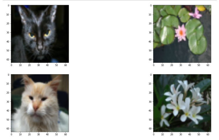
查看数据集中图片

import matplotlib.pyplot as plt
index = (25, 26, 27, 28)
plt.subplots(figsize=(20, 10))
for i in range(4):
    plt.subplot(2,2,i+1)
    plt.imshow(x_train[index[i]])

Result:

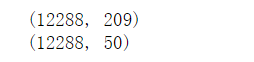
图片数组的处理

为了后面方便对数据的预测，我们将维度为(64, 64, 3)的数组重新构造为 (64x64x3, 1)的数组

x_train_flatten = x_train.reshape(x_train.shape[0], -1).T
# 这里.shape[]0]表示的是将第一维度作为新数组的第一维度，-1表示的是将剩下的维度相乘成为一个新的维度
x_test_flatten = x_test.reshape(x_test.shape[0], -1).T

查看新的数组形状

print(x_train_flatten.shape)

print(x_test_flatten.shape)

Result:

图片数据的处理

我们知道像素值处于0到255之间，为了后面数据处理的更加居中，我们将标准化的数据位于[0, 1]之间

X_train = x_train_flatten / 255.0
X_test = x_test_flatten / 255.0

构造logistic回归的梯度下降法

sigmoid函数

def sigmoid(z):
    s = 1 / (1 + np.exp(-z))
    return s

初始化w，b的函数

def initialize_w_b(dim):
    w = np.zeros(shape=(dim,1))
    
    b = 0
    assert(w.shape == (dim, 1))
    assert(isinstance(b, float) or isinstance(b, int)) # 在这里不写这个也是可以的，但是我们为了规范代码，避免不必要发生的错误，我们还是严谨一点
    
    return (w, b)
def initialize_w_b(dim):
    w = np.zeros(shape=(dim,1))
    
    b = 0
    assert(w.shape == (dim, 1))
    assert(isinstance(b, float) or isinstance(b, int)) # 在这里不写这个也是可以的，但是我们为了规范代码，避免不必要发生的错误，我们还是严谨一点
    
    return (w, b)

传播函数(propagate)

def propagate(w, b, X, Y):
    
    m = X.shape[1]
    # 正向传播
    z  = sigmoid(np.dot(w.T, X) + b)
    # 成本函数
    cost = (-1) * np.sum(Y * np.log(z) + (1 - Y) * (np.log(1 - z)))
    
    # 反向传播
    dw = (1 / m) * np.dot(X, (z- Y).T)
    db = (1/ m) * np.sum(z -  Y)
    
    assert(dw.shape == w.shape)
    assert(db.dtype == float)
    cost = np.squeeze(cost) # 将shape中为1的值剔除掉(即降维的处理)
    assert(cost.shape == ())
    # 字典存储 dw，db
    grads = {
        'dw':dw,
        'db':db
    }
    return (grads, cost)

优化函数

def  optimizer(w, b, X, Y, num_iterations, learning_rate,):
    costs = []
    
    for i in range (num_iterations):
        grads, cost = propagate(w, b, X, Y)
        
        dw = grads['dw']
        db = grads['db']
        # 更新w，b
        w = w - learning_rate * dw
        b = b - learning_rate * db
        
        if i % 100 == 0:
            costs.append(cost) # 存储成本函数的值
            print("迭代次数：i%，误差值：%f" % (i, cost))
            
    params = {
        'w':w,
        'b':b
    }
    grads ={
        'dw':dw,
        'db':db
    }
    return (params, grads, costs)

这样我们就完成了构造简单的logistic回归的梯度下降

预测函数

在模型进行预测的时候，我们可能会出现标签值位于(0,1)之间的值，为此我们需要进行下面的处理

def predict(w, b, X):
    m  = X.shape[1] #图片的数量
    Y_prediction = np.zeros((1,m)) 
    w = w.reshape(X.shape[0],1)
    
    #计预测猫在图片中出现的概率
    z = sigmoid(np.dot(w.T , X) + b)
    for i in range(z.shape[1]):
        #将概率z [0，i]转换为实际预测p [0，i]
        if z[0,i] > 0.5：
        	Y_prediction[0,i] = 1  
        else：
        	Y_prediction[0,i] = 0
    #使用断言
    assert(Y_prediction.shape == (1,m)) # 确保Y_prediction的形状
    return Y_prediction

我们就完成了我们需要的全部函数，最后写一个整合函数

整合函数

def model(X_train, Y_train, X_test, Y_test, num_iterations, learning_rate):
    w , b = initialize_w_b(X_train.shape[0])
    
    parameters , grads , costs = optimizer(w , b , X_train , Y_train,num_iterations , learning_rate)
    
    #从字典“参数”中检索参数w和b
    w , b = parameters["w"] , parameters["b"]
    
    #预测测试/训练集
    Y_prediction_test = predict(w , b, X_test)
    Y_prediction_train = predict(w , b, X_train)
    
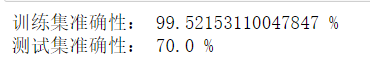
    #打印训练后的准确性
    print("训练集准确性："  , format(100 - np.mean(np.abs(Y_prediction_train - Y_train)) * 100) ,"%")
    print("测试集准确性："  , format(100 - np.mean(np.abs(Y_prediction_test - Y_test)) * 100) ,"%")
    
    stored = {
            "costs" : costs,
            "Y_prediction_test" : Y_prediction_test,
            "Y_prediciton_train" : Y_prediction_train,
            "w" : w,
            "b" : b,
            "learning_rate" : learning_rate,
            "num_iterations" : num_iterations }
    return stored

模型训练

d = model(X_train, y_train, X_test, y_test,num_iterations=2000, learning_rate=0.01)

Result:

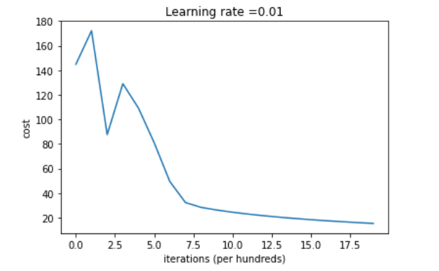
查看梯度下降学习的情况

costs = np.squeeze(d['costs'])
plt.plot(costs)
plt.ylabel('cost')
plt.xlabel('iterations ( hundreds)')
plt.title("Learning rate =" + str(d["learning_rate"]))
plt.show()

Result:

---

希望这篇文章对大家的学习有所帮助！