


干草垛(Haystack)里找“膝尖儿(Kneedle)”: 算法复现
缘起
-
引用:
Finding a “Kneedle” in a Haystack: Detecting Knee Points in System Behavior Ville Satopa † , Jeannie Albrecht† , David Irwin‡ , and Barath Raghavan§ †Williams College, Williamstown, MA ‡University of Massachusetts Amherst, Amherst, MA § International Computer Science Institute, Berkeley, CA
原文 图二: 粗图
def figure2():
    x = np.linspace(0.0, 1, 10)
    with np.errstate(divide='ignore'):
        return x,np.true_divide(-1, x + 0.1) + 5
x,y = figure2()
plt.plot(x,y)
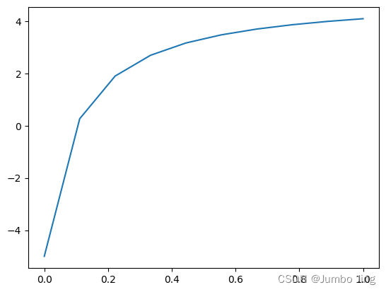
粗图: y = − 1 x + 0.1 + 5 y = \frac{-1}{x+0.1}+5 y=x+0.1−1+5
Step_1: 拟合条样曲线
from scipy.interpolate import interp1d # 用于插值的函数

N = len(x)

# Ds = 有限集合, 用于定义平滑曲线的x和y值, 该曲线已拟合平滑样条

uspline = interp1d(x, y) # 用x和y拟合样条曲线
Ds_y = uspline(x) # 样条曲线的y值

plt.plot(x, Ds_y);

拟合曲线
Step_2 曲线归一
def normalize(a):
    """返回归一化的array--`a`
    """
    return (a - min(a)) / (max(a) - min(a)) # 归一化, 使得a的最小值为0, 最大值为1
# x和y被归一到1x1的正方形中
x_normalized = normalize(x)
y_normalized = normalize(Ds_y)
Step_3 计算差异曲线
y_difference = y_normalized - x_normalized
x_difference = x_normalized.copy()

plt.title("Normalized spline & difference curve");
plt.plot(x_normalized, y_normalized);
plt.plot(x_difference, y_difference);
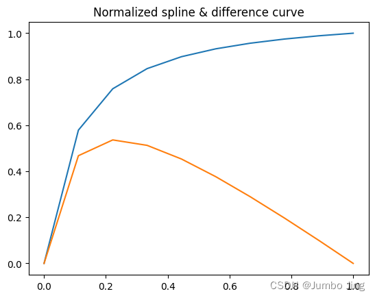
归一和差异曲线
Step_4 识别差异曲线的局部最大值
from scipy.signal import argrelextrema # 寻找局部最大值和最小值的函数

# 膝点是曲线中的局部最大值
maxima_indices = argrelextrema(y_difference, np.greater)[0] # 返回局部最大值的索引
x_difference_maxima = x_difference[maxima_indices] # 局部最大值的x值
y_difference_maxima = y_difference[maxima_indices] # 局部最大值的y值

# 局部最小值
minima_indices = argrelextrema(y_difference, np.less)[0]
x_difference_minima = x_difference[minima_indices]
y_difference_minima = y_difference[minima_indices]

plt.title("local maxima in difference curve");
plt.plot(x_normalized, y_normalized);
plt.plot(x_difference, y_difference);
plt.hlines(y_difference_maxima, plt.xlim()[0], plt.xlim()[1]);
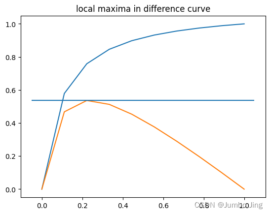
差异曲线局部最大值
Step_5 算阈值
# 敏感度参数`S`, 值越小, 膝点越快被检测到
S = 1.0

Tmx = y_difference_maxima \
    - (S * np.abs(np.diff(x_normalized).mean())) # 局部最大的阈值=局部最大值-x的平均差值*`S`
Step_6 找膝尖儿算法
"""
若差值曲线中的任何差值(xdj,ydj),其中j > i,
在下一个局部最大值被达到之前,下降到阈值y = T | mxi
对于(x | mxi,y | mxi),`
膝尖儿`在相应的x值处声明膝盖x = x | xi。
**如果差值达到局部最小值并在y = T | mxi之前开始增加,则将阈值值重置为0,并等待
达到另一个局部最大值。**

"""
# 人为地在x_difference数组的最后一项处放置局部最大值和局部最小值
maxima_indices = np.append(maxima_indices, len(x_difference) - 1)
minima_indices = np.append(minima_indices, len(x_difference) - 1)

# 阈值区域i所在的占位符。
maxima_threshold_index = 0
minima_threshold_index = 0

curve = 'concave'
direction = 'increasing'

all_knees = set() # 所有膝点的集合
all_norm_knees = set() # 所有归一化膝点的集合

# 遍历差分曲线
for idx, i in enumerate(x_difference):

    # 到达曲线的尽头
    if i == 1.0:
        break

    if idx >= maxima_indices[maxima_threshold_index]:
        threshold = Tmx[maxima_threshold_index]
        threshold_index = idx
        maxima_threshold_index += 1

    # 差值曲线中的值处于局部最小值或之后
    if idx >= minima_indices[minima_threshold_index]:
        threshold = 0.0
        minima_threshold_index += 1

    # 不要在第一个局部最大值之前评估差异曲线中的值。
    if idx < maxima_indices[0]:
        continue

    # 评估阈值
    if y_difference[idx] < threshold:
        if curve == 'convex':
            if direction == 'decreasing':
                knee = x[threshold_index]
                all_knees.add(knee)
                norm_knee = x_normalized[threshold_index]
                all_norm_knees.add(norm_knee)
            else:
                knee = x[-(threshold_index + 1)]
                all_knees.add(knee)
                norm_knee = x_normalized[-(threshold_index + 1)]
                all_norm_knees.add(norm_knee)

        elif curve == 'concave':
            if direction == 'decreasing':
                knee = x[-(threshold_index + 1)]
                all_knees.add(knee)
                norm_knee = x_normalized[-(threshold_index + 1)]
                all_norm_knees.add(norm_knee)
            else:
                knee = x[threshold_index]
                all_knees.add(knee)
                norm_knee = x_normalized[threshold_index]
                all_norm_knees.add(norm_knee)
#%%
plt.xticks(np.arange(0,1.1,0.1))
plt.plot(x_normalized, y_normalized);
plt.plot(x_difference, y_difference);
plt.plot(all_norm_knees, y_normalized, 'o');
plt.hlines(Tmx[0], plt.xlim()[0], plt.xlim()[1], colors='g', linestyles='dashed');
plt.vlines(x_difference_maxima, plt.ylim()[0], plt.ylim()[1], colors='r', linestyles='dashed');
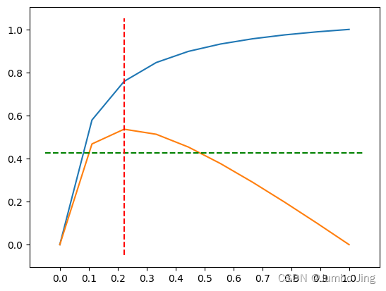
垂直的红色虚线表示拐点的x值。水平的绿色虚线表示阈值。
理解和不解:
原文 里面写了好多个公式, 代码却这么简单(当然也有一些不解)
- 具体到算法无非是归一后, 再归一, 也就是说–先将x和y归一, 再将y-x…
- 原文里面的那些公式呢?代码里面没体现呀…
- 就这些吧…搬过来将就用


 1933
1933

 被折叠的 条评论
为什么被折叠?
被折叠的 条评论
为什么被折叠?
 到【灌水乐园】发言


