深度学习PyTorch（二）卷积神经网络

背景及应用

基础及计算

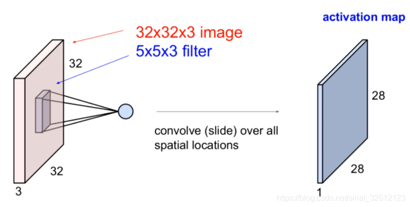
因为是彩色图片，所以有RGB三个通道。

传统方法处理图像

卷积

引入卷积
十字架元素不等于零。

卷积运算
左边的矩阵是输入图像抽取的一部分，表示每一个像素点的像素值。

卷积运算
到
运算规则


卷积

扩充0来增加卷积输出的大小：



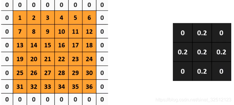
以上输出矩阵从4×4到6×6，还可以保留边缘信息。原本边缘信息只能用到一次，用这个方法可以用到很多次。
我们在矩阵外部补零的时候可以补很多层0，称这个层数为“padding”
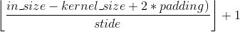
卷积输出后矩阵大小的计算公式（以宽度为例）
$W_{out}=(W-K+2P)/S+1$，有小数，则向下取整。


卷积层

比如：输入（32，32，3）的矩阵，有6个（5，5）卷积核。
那么我们就有5个（28，28）输出矩阵，连接起来就是（28，28，6）的输出
总结

池化

找最大值输出：最大值池化
统计平均值信息：均值池化

池化的作用

计算公式和卷积一样，但如果有小数，向上取整。

感受野

感受野计算时有下面几个知识点需要知道：

. 最后一层（卷积层或池化层）输出特征图感受野的大小等于卷积核的大小。
. 第i层卷积层的感受野大小和第i层的卷积核大小和步长有关系，同时也与第（i+1）层感受野大小有关。
. 计算感受野的大小时忽略了图像边缘的影响，即不考虑padding的大小。
关于感受野大小的计算方式是采用从最后一层往下计算的方法，即先计算最深层在前一层上的感受野，然后逐层传递到第一层，使用的公式可以表示如下：

其中，$R{F}_i$是第i层卷积层的感受野，$R{F}_{i+1}$是（i+1）层上的感受野，stride是卷积的步长，Ksize是本层卷积核的大小。

卷积神经网络的定义bvb

是一个"卷积层"+“池化层”，
作为神经网络的隐藏层反复出现的多层神经网络结构。

CNN在pytorch中的实现

ReLU(inplace=True)
inplace=True
计算结果不会有影响。利用in-place计算可以节省内（显）存，同时还可以省去反复申请和释放内存的时间。但是会对原变量覆盖，只要不带来错误就用。
inplace为True，将会改变输入的数据 ，否则不会改变原输入，只会产生新的输出

卷积：

pytorch中有函数torch.nn.Con2d()来实现卷积
和torch.nn.functional.con2d()两种实现方式


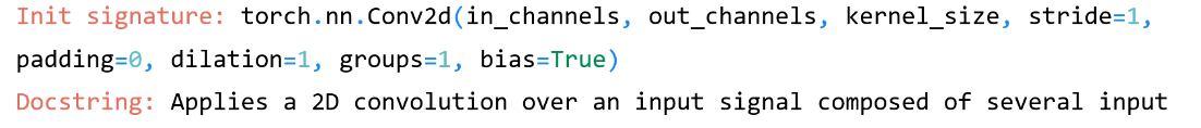
dilation(扩张)：控制kernel点（卷积核点）的间距; 也被称为 "à trous"算法. 可以在此github地址查看:Dilated convolution animations
groups(卷积核个数)：这个比较好理解，通常来说，卷积个数唯一，但是对某些情况，可以设置范围在1 —— in_channels中数目的卷积核

bias:默认为True，表示使用偏置
groups：groups=1表示所有输入输出是相关联的；groups=n表示输入输出通道数（深度）被分割为n份，并分别对应，且需要被groups整除
（dilation:卷积对输入的空间间隔，默认为dilation=1）

卷积输入为torch.autograd.Variable()的类型，大小为（batch，channel，H，W）

卷积实例
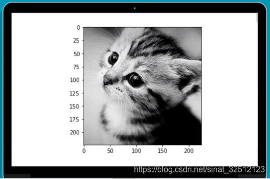
输入图片：

"""
在Pytorch中定义一个能够检测边缘的卷积核
"""
import numpy as np
import torch
from torch import nn
from torch.autograd import Variable
import torch.nn.functional as F
from PIL import Image
import matplotlib.pyplot as pt
#%matplotlib inline

im=Image.open('./cat.png').convert('L')#转化为灰度图
im=np.array(im,dtype=float32)

#可视化图片
plt.imshow(im.astype('unit8'),cmp='gray')

#将图片矩阵转化为pytorch tensor,并适配卷积输入的要求
im=im.reshape((1,1,im.shape[0],im.reshape[1]))#in,out,H,W
im=torch.from_numpy(im)

#定义一个算子对其进行轮廓检测
# 使用nn.conv2f
conv1=nn.Conv2d(1,1,3,bias=False)#定义卷积

sobel_kernel=np.array([[-1,-1,-1],[-1,8,-1],[-1,-1,-1]],dtype=='float32')#定义轮廓检测算子
sobel_kernel=sobel_kernel.reshape((1,1,3,3))#适配卷积的输入输出
conv1.weight.data=torch.from_numpy(sobel_kernel)#给卷积的kernel赋值

edge1=conv1(Variable(im))#作用在图片上
edge1=edge1.data.squeeze().numpy()#将输出转换为图片的形式,删除所有单维度的条目

plt.imshow(edge1,cmap='gray')

# 使用nn.function.conv2d
sobel_kernel=np.array([[-1,-1,-1],[-1,8,-1],[-1,-1,-1]],dtype=='float32')#定义轮廓检测算子
sobel_kernel=sobel_kernel.reshape((1,1,3,3))#适配卷积的输入输出
weight=Variable(torch.from_numpy(sobel_kernel))

edge2=F.conv2d(Variable(im),weight)#作用在图片上
edge2=edge2.data.squeeze().numpy()#将输出转化为图片的格式

plt.imshow(edg2,cmp='gray')

结果图：

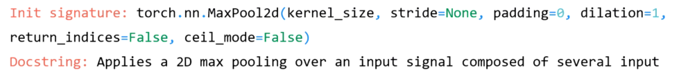
池化:

pytorch中有函数torch.nn.MaxPool2d()或者torch.nn.functional.max_pool2d()来实现最大值池化

#使用nn.MaxPool2d
print('before max pool,image shape:{}*{}'.format(im.shape[2],im.shape[3]))
pool=nn.MaxPool2d(2,2)#kernel_size=2*2，stride=2
small_im1=pool(Variable(img))
small_im1=small_im1.data.squeeze().numpy()
print('after max pool,image shape:{}*{}'.format(small_im1.shape[0],small_im1.shape[0]))
plt.imshow(small_im1,cmap='gray')

#使用F.max_pool2d()
print('before max pool,image shape:{}*{}'.format(im.shape[2],im.shape[3]))
smal2_im1=F.max_pool2d(Variable(img),2,2)
smal2_im1=small_im1.data.squeeze().numpy()
print('after max pool,image shape:{}*{}'.format(small_im1.shape[0],small_im1.shape[0]))
plt.imshow(small_im2,cmap='gray')

结果：

before max pool, image shape: 224 x 224
after max pool, image shape: 112 x 112

结果图：

Numpy中ndim、shape、dtype、astype的用法

标准化

对数据增加预处理，同时使用批标准化能够得到非常好的收敛结果，这也是卷积网络能够训练到非常深的层的一个重要原因。

数据预处理

尽量输入特征不相关且满足一个标准的正态分布。
最常见的方法是中心化和标准化。
中心化
修正数据的中心位置。
实现方法：在每个特征维度上减去对应的均值，最后得到0均值的特征。
标准化
把数据变成0均值后，为了使得不同的特征维度有相同的规模，除以标准差近似为一个标准正态分布。
也可以依据最大值和最小值将其转化为-1~1之间。

另外有些方法，比武PCA或者白噪声已经用的非常少了。

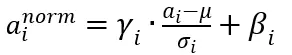
Batch Normalization

对于很深的网路结构，网路的非线性层会使得输出的结果变得相关，且不再满足一个标准的B(0,1)分布，甚至输入的中心已经发生偏移，这对于训练深层模型是很不有利的。

BN是对每一层网络的输出，做一个归一化，使其服从标准的正态分布。从而加快收敛。

实现：
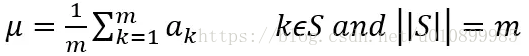
对于给定的一个batch的数据 B = { x 1 , x 2 , . . . , x m } {B =\{ {x_1},{x_2},...,{x_m}\}} B={x1​,x2​,...,xm​}算法 的公式如下：

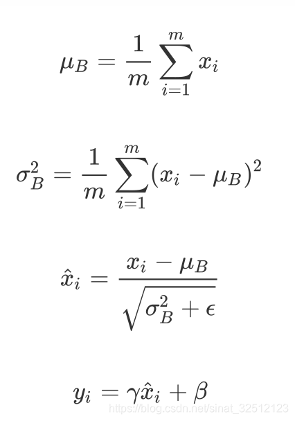
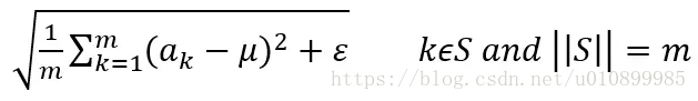
1.第一行和第二行是计算出一个batch中数据的均值和方差
2.接着使用第三个公式对batch中的每个数据点做标准化，$\epsilon$是为了计算稳定引入的一个小的常数，通常取 $10^{-5}$。
3.最后利用权重修正得到最后的输出结果

有名的卷积网络结构

2010年ILSVRC 1000分类

数据集：CIFAR 10

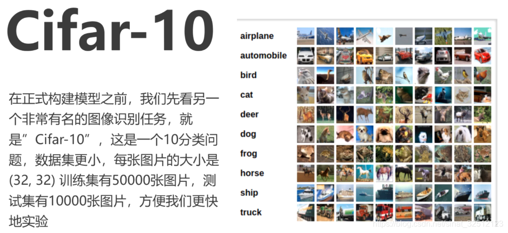
AlexNet

8层CNN

几个卷积池化堆叠后连接几个全连接层
结构图

pytorch实现

将矩阵拉平,torch中的view相当于numpy中的reshape
x=x.reshape((-1,))

import torch
from torch import nn
import numpy as np
from torch.autograd import Variable
from torchvision.datasets import CIFIR10
from utils import train

class AlexNet(nn.Modele):
    def __init__(self):
        super(AlexNet,self).__init__()
        #第一层是5*5的卷积，输入的channels是3，输出的channels是64，步长是1，没有padding
        self.conv1=nn.Sequential(
            nn.Conv2d(3,64,5),#（32-5）+1=28(64,28,28)
            nn.ReLU(True)
        )

        #第二层是3*3的池化，步长是2，没有padding
        self.max_pool1=nn.MaxPool2d(3,2)#(28-3)/2+1=13 (64,13,13)

        #第三层是5*5的卷积，输入的channel是64，输出的channel是64，步长为1，没有padding
        self.conv2=nn.Sequential(
            nn.Conv2d(64,64,5),#(13-5)+1=9,(64,9,9)
            nn.ReLU(True)
        )

        #第四层是3*3的池化，步长是2，没有padding
        self.max_pool2=nn.MaxPool2d(3,2)#(9-3)/2+1=4,(64,4,4)

        #第五层是全连接层，输入是1204，输出是384
        self.fc1=nn.Sequential(
            nn.Linear(1024,384),
            nn.ReLU(True)
        )

        # 第五层是全连接层，输入是384，输出是192
        self.fc2 = nn.Sequential(
            nn.Linear(384, 192),
            nn.ReLU(True)
        )

        # 第六层是全连接层，输入是192，输出是10
        self.fc2 = nn.Sequential(
            nn.Linear(192,10)
        )
    def forward(self,x):
        x=self.conv1(x)
        x=self.max_pool1(x)
        x = self.conv2(x)
        x = self.max_pool2(x)

        #将矩阵拉平,torch中的view相当于numpy中的reshape
        x=x.view(x.shape[0],-1)
        x = self.fc1(x)
        x = self.fc2(x)
        x = self.fc3(x)
        return x

alexnet=AlexNet()
#为验证网络结构是否正确，先输入一张32*32的图片，看看输出
#定义输入为（1，3，32，32）
input_demo=Variable(torch.zeros(1,3,32,32))
out_demo=alexnet(input_demo)
print(out_demo,shape)#torch.size([1,10])

def data_tf(x):
    x=np.arrar(x,dtype='float')/255
    x=(x-0.5)/0.5#标准化
    x.transpose(2,0,1)#将channel放到第一维，只是pytorch要求地输入方式
    x=torch.from_numpy(x)
    return x

train_set=CIFIR10('./data',train=True,transform=data_tf)
test_set=CIFIR10('./data',train=False,transform=data_tf)
train_data=torch.utils.data.DataLoader(train_set,batch_size=64,shufflr=True)
test_data=torch.utils.data.DataLoader(test_set,batch_size=128,shufflr=True)

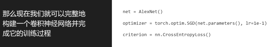
net=AlexNet()
optimizer=torch.optim.SGD(net.parameters(),lr=1e-1)
criterion=nn.CrossEntropyLoss()

train(net,train_data,test_data,20,optimizer,criterion)#训练20次

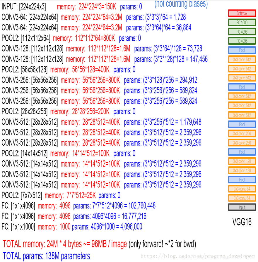
VGG

第一个真正意义上的深层神经网络结构，是ImageNet2014年的亚军。
得益于python函数和循环，能方便地构建重复结构的深层网络。

不断地堆叠卷积层和池化层。
几乎全部使用3×3的卷积核和2×2的池化层 。
作用：使用小的卷积核进行多层的堆叠和一个大的卷积核的感受野是相同的，同时小的卷积核还能减少参数，同时可以有更深的结构。
关键：使用很多层的3×3的卷积核然后再使用一个最大池化层。这个模块使用很多次。
第一层是11×11的卷积，96个核，步长stride=4,最大值池化，图像大小会减小一半。

pytorch实现

import torch
from torch import nn
import numpy as np
from torch.autograd import Variable
from torchvision.datasets import CIFIR10
from utils import train

def vgg_block(num_convs,in_channels,out_channels):
    net=[nn.Conv2d(in_channels,out_channels,kernel_size=3,padding=1),#(300-3+2)/1+1=300
         nn.ReLU(True)]#定义第一层
    for i in range(num_convs-1):#定义后面的很多层
        net.append(nn.Conv2d(out_channels,out_channels,kenel_size=3,padding=1))#(300-3+2)+1=300
        net.append(ReLU(True))                                                  #(300-3+2)+1=300
    net.append(nn.MaxPool2d(2,2))#定义池化层(300-2)/2+1=150
    return nn.Sequential(*net)

#将模型打印出来看结构
block_demo=vgg_block(3,64,128)
print(block_demo)
"""
结果;
Sequential(
(0): Conv2d (64, 128, kernel_size=(3, 3), stride=(1, 1), padding=(1, 1))
(1): ReLU(inplace)
(2): Conv2d (128, 128, kernel_size=(3, 3), stride=(1, 1), padding=(1, 1))
(3): ReLU(inplace)
(4): Conv2d (128, 128, kernel_size=(3, 3), stride=(1, 1), padding=(1, 1))
(5): ReLU(inplace) 
(6): MaxPool2d(kernel_size=(2, 2), stride=(2, 2), dilation=(1, 1))
)
"""
#首先定义输入为（1，64，300，300）
input_demo=Variable(torch.zeros(1,64,300,300))#（batch.out_channel,H,W）
output_demo=block_demo(input_demo)
print(out_demo.shape)#torch.Size([1, 128, 150, 150])?

#定义一个函数对vgg bolck堆叠
def vgg_stack(num_convs,channels):
    net=[]
    # zip() 函数用于将可迭代的对象作为参数，将对象中对应的元素打包成一个个元组，然后返回由这些元组组成的列表
    for n,c in zip(num_convs,channels):
        int_c=c[0]
        out_c=c[1]
        net.append(vgg_block(n,int_c,out_c))
    return nn.Sequential(*net)

#定义一个简单点的VGG结构，8个卷积层进行测试。
vgg_net=vgg_stack((1,1,2,2,2),((3,64),(64,128),(128,256),(256,512),(512,512)))
print(vgg_net)

"""
Sequential(
(0): Sequential(
(0): Conv2d (3, 64, kernel_size=(3, 3), stride=(1, 1), padding=(1, 1))
(1): ReLU(inplace)
(2): MaxPool2d(kernel_size=(2, 2), stride=(2, 2), dilation=(1, 1))
)
(1): Sequential(
(0): Conv2d (64, 128, kernel_size=(3, 3), stride=(1, 1), padding=(1, 1))
(1): ReLU(inplace)
(2): MaxPool2d(kernel_size=(2, 2), stride=(2, 2), dilation=(1, 1))
)
(2): Sequential(
(0): Conv2d (128, 256, kernel_size=(3, 3), stride=(1, 1), padding=(1, 1))
(1): ReLU(inplace)
(2): Conv2d (256, 256, kernel_size=(3, 3), stride=(1, 1), padding=(1, 1))
(3): ReLU(inplace)
(4): MaxPool2d(kernel_size=(2, 2), stride=(2, 2), dilation=(1, 1))
)
(3): Sequential(
(0): Conv2d (256, 512, kernel_size=(3, 3), stride=(1, 1), padding=(1, 1))
(1): ReLU(inplace)
(2): Conv2d (512, 512, kernel_size=(3, 3), stride=(1, 1), padding=(1, 1))
(3): ReLU(inplace)
(4): MaxPool2d(kernel_size=(2, 2), stride=(2, 2), dilation=(1, 1))
)
(4): Sequential(
(0): Conv2d (512, 512, kernel_size=(3, 3), stride=(1, 1), padding=(1, 1))
(1): ReLU(inplace)
(2): Conv2d (512, 512, kernel_size=(3, 3), stride=(1, 1), padding=(1, 1))
(3): ReLU(inplace)
(4): MaxPool2d(kernel_size=(2, 2), stride=(2, 2), dilation=(1, 1))
)
)
"""
#可以看出该网络有5个池化层，图片大小会减少2^5倍。测试：
test_x=Variable(torch.zeros(1,3,256,256))
test_y=vgg_net(test_x)
print(test_y,shape)# torch.Size([1, 512, 8, 8])

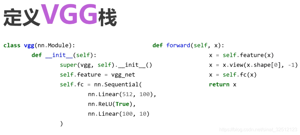
class vgg(nn.Modele):
    def __init__(self):
        super(vgg,self).__init__()
        self.feature=vgg_net
        self.fc=nn.Sequential(
            nn.Linear(512,100),
            nn,ReLU(),
            nn.Linear(100,10)
        )
        
    def forward(self,x):
        x=self.feature(x)
        #将矩阵拉平,torch中的view相当于numpy中的reshape
        x=x.view(x.shape[0],-1)
        x = self.fc(x)
        return x

def data_tf(x):
    x=np.arrar(x,dtype='float')/255
    x=(x-0.5)/0.5#标准化
    x.transpose(2,0,1)#将channel放到第一维，只是pytorch要求地输入方式
    x=torch.from_numpy(x)
    return x

train_set=CIFIR10('./data',train=True,transform=data_tf)
test_set=CIFIR10('./data',train=False,transform=data_tf)
train_data=torch.utils.data.DataLoader(train_set,batch_size=64,shufflr=True)
test_data=torch.utils.data.DataLoader(test_set,batch_size=128,shufflr=True)

net=net=vgg()
optimizer=torch.optim.SGD(net.parameters(),lr=1e-1)
criterion=nn.CrossEntropyLoss()

train(net,train_data,test_data,20,optimizer,criterion)#训练20次

GoogLeNet

ImageNet2014年的冠军。
颠覆了传统卷积网络的串联的印象和固定做法，采用了一种非常有效的inception模块，得到了比VGG更深的网络结构，却比 VGG的参数更少，因为去掉了后面的全连接层，所以参数大大减少，同时有了很高的计算效率。
加入了更加结构化的Inception块使得我们能够使用更大的通道，更多的层，同时控制了计算量。
Inception模块:四个并行卷积的层。

最后将四个并行线路得到的特征在通道这个维度上拼接在一起。


从左到右：
第一分支：不同感受野
第二分支：减少通道数，扩大感受野
……
得到四个不同的特征

pytorch实现

原论文使用多个输出来解决梯度小时的问题，这里我们之定义一个简单版本的GooLeNet，简化一个输出。

import numpy as np
import torch
from torch import nn
from torch.autograd import Variable
from torchvision.datasets import CIFAR10
from utils import train

#定义一个卷积加一个relu激活函数和一个batchnorm作为一个基本的层的结构
def conv_relu(in_channels,out_channels,kernel,stride=1,padding=0,):
    layer=nn.Sequential(
        nn.Conv2d(in_channels,out_channels,kernel,stride,padding),
        nn.BatchNorm2d(out_channels,eps=1e-3),
        nn.ReLU(True)
    )
    return layer

class inception(nn.Module):
    def __init__(self,in_channel,out1_1,out2_1,out2_3,out3_1,out3_5,out4_1):
        super(inception,self).__init__()
        #第一条线路
        self.batch1x1=conv_relu(in_channel,out1_1,1)

        #第二条线路
        self.batch3x3=nn.Sequential(
            conv_relu(in_channel,out2_1,1),
            conv_relu(out2_1,out2_3,3,padding=1)
        )

        # 第三条线路
        self.batch5x5 = nn.Sequential(
            conv_relu(in_channel, out3_1, 1),
            conv_relu(out2_1, out3_5, 5,padding=2)
        )

        # 第四条线路
        self.batch_pool = nn.Sequential(
            nn.MaxPool2d(3,stride=1,padding=1),
            conv_relu(out2_1, out4_1, 1)
        )
    def forward(self,x):
        f1=self.batch1x1(x)
        f2=self.batch3x3(x)
        f3=self.batch5x5(x)
        f4=self.batch_pool(x)
        out=torch.cat((f1,f2,f3,f4),dim=1)#按行拼接在后面
        return out
#测试：
test_net=inception(3,64,48,64,64,96,32)
test_x=Variable(torch.zeros(1,3,96,96))
print('input shape: {} x {} x {}'.format(test_x.shape[1], test_x.shape[2],test_x.shape[3]))
test_y = test_net(test_x)
print('output shape: {} x {} x {}'.format(test_y.shape[1], test_y.shape[2],test_y.shape[3]))

"""
input shape: 3 x 96 x 96
output shape: 256 x 96 x 96
#大小没有发生变化，通道维数变多
"""

class googlenet(nn.Module):
    def __init__(self, in_channel, num_classes, verbose=False):
        super(googlenet, self).__init__()
        self.verbose = verbose

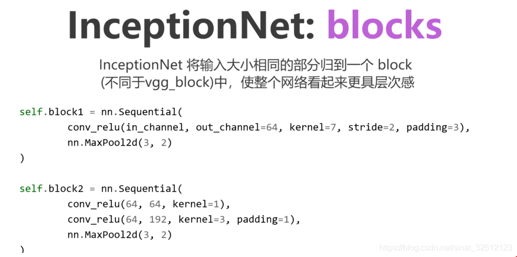
        self.block1 = nn.Sequential(
        conv_relu(in_channel, out_channel=64, kernel=7, stride=2, padding=3),
        nn.MaxPool2d(3, 2)
        )
        self.block2 = nn.Sequential(
        conv_relu(64, 64, kernel=1),
        conv_relu(64, 192, kernel=3, padding=1),
        nn.MaxPool2d(3, 2)
        )
        self.block3 = nn.Sequential(
        inception(192, 64, 96, 128, 16, 32, 32),
        inception(256, 128, 128, 192, 32, 96, 64),
        nn.MaxPool2d(3, 2)
        )
        self.block4 = nn.Sequential(
        inception(480, 192, 96, 208, 16, 48, 64),
        inception(512, 160, 112, 224, 24, 64, 64),
        inception(512, 128, 128, 256, 24, 64, 64),
        inception(512, 112, 144, 288, 32, 64, 64),
        inception(528, 256, 160, 320, 32, 128, 128),
        nn.MaxPool2d(3, 2)
        )
        self.block5 = nn.Sequential(
        inception(832, 256, 160, 320, 32, 128, 128),
        inception(832, 384, 182, 384, 48, 128, 128),
        nn.AvgPool2d(2)
        )
        self.classifier = nn.Linear(1024, num_classes)

    def forward(self, x):
        x = self.block1(x)
        if self.verbose:
            print('block 1 output: {}'.format(x.shape))
        x = self.block2(x)
        if self.verbose:
            print('block 2 output: {}'.format(x.shape))
            x = self.block3(x)
            if self.verbose:
                print('block 3 output: {}'.format(x.shape))
            x = self.block4(x)
            if self.verbose:
                print('block 4 output: {}'.format(x.shape))
            x = self.block5(x)
            if self.verbose:
                print('block 5 output: {}'.format(x.shape))
            x = x.view(x.shape[0], -1)
            x = self.classifier(x)
            return x

test_net = googlenet(3, 10, True)
test_x = Variable(torch.zeros(1, 3, 96, 96))
test_y = test_net(test_x)
print('output: {}'.format(test_y.shape))

"""
block 1 output: torch.Size([1, 64, 23, 23])
block 2 output: torch.Size([1, 192, 11, 11])
block 3 output: torch.Size([1, 480, 5, 5])
block 4 output: torch.Size([1, 832, 2, 2])
block 5 output: torch.Size([1, 1024, 1, 1])
output: torch.Size([1, 10])
输入的尺寸不断减少，通道的维数不断增加
"""

def data_tf(x):
    x = x.resize((96, 96), 2) # 将图片放大到 96 x 96，resize(size,interpolation=2)
    x = np.array(x, dtype='float32') / 255
    x = (x - 0.5) / 0.5 # 标准化
    x = x.transpose((2, 0, 1)) # 将channel放到第一维
    x = torch.from_numpy(x)
    return x

train_set = CIFAR10('./data', train=True, transform=data_tf)
train_data = torch.utils.data.DataLoader(train_set, batch_size=64, shuffle=True)
test_set = CIFAR10('./data', train=False, transform=data_tf)
test_data = torch.utils.data.DataLoader(test_set, batch_size=128, shuffle=False)

net = googlenet(3, 10)
optimizer = torch.optim.SGD(net.parameters(), lr=0.01)
criterion = nn.CrossEntropyLoss()
train(net, train_data, test_data, 20, optimizer, criterion)

ResNet

ImageNet2015年的冠军。
使用跨层通道使得训练非常深的卷积神经网络成为可能。同样它使用非常简单的卷积层配置，使得其拓展更加简单。

pytorch实现

import numpy as np
import torch
from torch import nn
import torch.nn.functional as F
from torch.autograd import Variable
from torchvision.datasets import CIFAR10
from utils import train

def conv3x3(in_channel,out_channel,stride=1):
    return nn.Conv2d(in_channel,out_channel,3,stride=stride,padding=1,bias=False)

class residual_block(nn.Module):
    def __init__(self,in_channel,out_channel,same_shape=True):
        super(residual_block,self).__init__()
        self.same_shape=same_shape
        stride=1 if self.same_shape else 2

        self.conv1=conv3x3(in_channel,out_channel,stride=stride)
        stride = 1 if self.same_shape else 2

        self.conv2 = conv3x3(out_channel, out_channel)
        self.bn1=nn.BatchNorm2d(out_channel)
        if not self.same_shape:
            self.conv3=nn.conv2d(in_channel,out_channel,1,stride=stride)

    def forward(self, x):
        out = self.conv1(x)
        out = F.relu(self.bn1(out), True)
        out = self.conv2(out)
        out = F.relu(self.bn2(out), True)
        if not self.same_shape:
            x = self.conv3(x)
        return F.relu(x + out, True)

#测试输出
#输入输出形状相同
test_net = residual_block(32, 32)
test_x = Variable(torch.zeros(1, 32, 96, 96))
print('input: {}'.format(test_x.shape))
test_y = test_net(test_x)
print('output: {}'.format(test_y.shape))

"""
input: torch.Size([1, 32, 96, 96])
output: torch.Size([1, 32, 96, 96])
"""

#输入输出形状不同
test_net = residual_block(3, 32, False)
test_x = Variable(torch.zeros(1, 3, 96, 96))
print('input: {}'.format(test_x.shape))
test_y = test_net(test_x)
print('output: {}'.format(test_y.shape))
"""
input: torch.Size([1, 3, 96, 96])
output: torch.Size([1, 32, 48, 48])
"""

class resnet(nn.Module):
    def __init__(self, in_channel, num_classes, verbose=False):
        super(resnet, self).__init__()
        self.verbose = verbose
        self.block1 = nn.Conv2d(in_channel, 64, 7, 2)
        self.block2 = nn.Sequential(
        nn.MaxPool2d(3, 2),
        residual_block(64, 64),
        residual_block(64, 64)
        )
        self.block3 = nn.Sequential(
        residual_block(64, 128, False),
        residual_block(128, 128)
        )
        self.block4 = nn.Sequential(
        residual_block(128, 256, False),
        residual_block(256, 256)
        )
        self.block5 = nn.Sequential(
        residual_block(256, 512, False),
        residual_block(512, 512),
        nn.AvgPool2d(3)
        )
        self.classifier = nn.Linear(512, num_classes)

    def forward(self, x):
        x = self.block1(x)
        if self.verbose:
            print('block 1 output: {}'.format(x.shape))
        x = self.block2(x)
        if self.verbose:
            print('block 2 output: {}'.format(x.shape))
        x = self.block3(x)
        if self.verbose:
            print('block 3 output: {}'.format(x.shape))
        x = self.block4(x)
        if self.verbose:
                print('block 4 output: {}'.format(x.shape))
        x = self.block5(x)
        if self.verbose:
                print('block 5 output: {}'.format(x.shape))
        x = x.view(x.shape[0], -1)
        x = self.classifier(x)
        return x

#测试
test_net = resnet(3, 10, True)
test_x = Variable(torch.zeros(1, 3, 96, 96))
test_y = test_net(test_x)
print('output: {}'.format(test_y.shape))

"""
block 1 output: torch.Size([1, 64, 45, 45])
block 2 output: torch.Size([1, 64, 22, 22])
block 3 output: torch.Size([1, 128, 11, 11])
block 4 output: torch.Size([1, 256, 6, 6])
block 5 output: torch.Size([1, 512, 1, 1])
output: torch.Size([1, 10])
"""

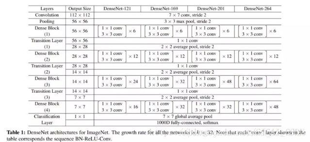
DenseNet

cvpr2017 best paper
DenseNet将残差连接改为了特征拼接，使网络有了更稠密的连接
ResNet跨层连接的思想影响了后面很多网络。

pytorch实现

import numpy as np
import torch
from torch import nn
from torch.autograd import Variable
from torchvision.datasets import CIFAR10
from utils import train

"""
首先定义一个卷积快，卷积块的顺序为bn,relu,conv
"""
def conv_block(in_channel,out_channel):
    layer=nn.Sequential(
        nn.BatchNorm2d(in_channel),
        nn.ReLU(True),
        nn.Conv2d(in_channel,out_channel,3,padding=1,bias=False)
    )
    return layer

"""
dense block将每次的卷积输出称为growth_rate，如果输入时in_channel，有n层，那么输出就是in_channel+n*growth_rate
"""
class dense_block(nn.Module):
    def __init__(self,in_channel,growth_rate,num_layers):
        block=[]
        channel=in_channel
        for i in range(num_layers):
            block.append(conv_block(channel,growth_rate))
            channel+=growth_rate

        self.net=nn.Sequential(*block)

    def forward(self,x):
        for layer in self.net:
            out=layer(x)
            x=torch.cat((out,x),dim=1)
        return x

#验证输出的channel对不对
test_net = dense_block(3, 12, 3)
test_x = Variable(torch.zeros(1, 3, 96, 96))
print('input shape: {} x {} x {}'.format(test_x.shape[1], test_x.shape[2],test_x.shape[3]))
test_y = test_net(test_x)
print('output shape: {} x {} x {}'.format(test_y.shape[1], test_y.shape[2],test_y.shape[3]))
"""
input shape: 3 x 96 x 96
output shape: 39 x 96 x 96
"""

"""
因为DenseNet会不断对维数进行拼接，当层数越高时，输出通道数越来越大，参数和计算量也越来越大。
为了避免这个问题，需要引入过渡层将输出通道降低下来，同时将输入的长宽减半，这个过渡层可以使用1*1的卷积
transition block
"""
def transition_block(in_channel,out_channel):
    trans_layer=nn.Sequential(
        nn.BatchNorm2d(in_channel),
        nn.ReLU(True),
        nn.Conv2d(in_channel,out_channel,1),
        nn.AvgPool2d(2,2)
    )
    return trans_layer

#验证过渡层是否正确
test_net = transition_block(3, 12)
test_x = Variable(torch.zeros(1, 3, 96, 96))
print('input shape: {} x {} x {}'.format(test_x.shape[1], test_x.shape[2],test_x.shape[3]))
test_y = test_net(test_x)
print('output shape: {} x {} x {}'.format(test_y.shape[1], test_y.shape[2],test_y.shape[3]))
"""
input shape: 3 x 96 x 96
output shape: 12 x 48 x 48
"""

class densenet(nn.Module):
    def __init__(self,in_channel,num_classes,growth_rate=32,block_layers=[6,12,24,16]):
        super(densenet,self).__init__()
        self.block1=nn.Sequential(
            nn.Conv2d(in_channel, 64, 7, 2, 3),
            nn.BatchNorm2d(64),
            nn.ReLU(True),
            nn.MaxPool2d(3, 2, padding=1)
        )

        channels=64
        block=[]
        for i,num_layers in enumerate(block_layers):
            block.append(dense_block(channels,growth_rate,num_layers))
            channels+=growth_rate
            if i!=num_layers-1:
                block.append(transition_block(channels,channels//2))#大小减半，通道数减半
                channels=channels//2
        self.block2=nn.Sequential(*block)
        self.block2.add_module('bn',nn.BatchNorm2d(channels))
        self.block2.add_module('relu',nn.ReLU(True))
        self.block2.add_module('adg_pool',nn.AvgPool2d(3))

        self.classifier=nn.Linear(channels,num_classes)

    def forward(self,x):
        x=self.block1(x)
        x=self.block2(x)
        x=x.view(x.shape[0],-1)
        x=self.classifier(x)
        return  x

#测试
test_net = densenet(3, 10)
test_x = Variable(torch.zeros(1, 3, 96, 96))
test_y = test_net(test_x)
print('output: {}'.format(test_y.shape))
#output: torch.Size([1, 10])

卷积神经网络训练技巧

欠拟合：模型训练次数还不够或者模型太简单，没有拟合好真实的数据。
解决办法:进行充分训练，或者增加模型的复杂度。

过拟合：在训练集表现良好，但在测试集上表现不好。以下时减小过拟合的方法。

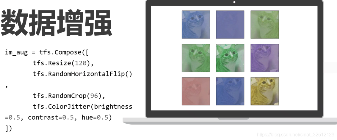
数据增强

对训练数据进行扩充的方法，使模型具有不错的表达能力和泛化能力。
当数据量不足时，模型陷入局部最优解、出现过拟合等现象。

from PIL import Image
from torchvision import transforms as tfs

#读入一张图片
im=Image.open('./cat.png')

"""
比例缩放 tfs.Resize(）
第一个参数可以是一个整数，图片会保存现在的宽和高的比例，并将更短的边缩放到这个整数的大小。
第一个参数可以是一个tuple(元组)，图片会直接把宽和高缩放到这个大小。
第二个参数表示放缩图片使用的方法，比如最近邻法，双线性差值。默认双线性差值，因其能保留图片更多信息
"""
#比例缩放
print('before scale, shape: {}'.format(im.size))
new_im=tfs.Resize((100,200))(im)
print('after scale, shape: {}'.format(new_im.size))
"""
before scale, shape: (224, 224)
after scale, shape: (200, 100)
"""

"""
随机位置截取 
tfs.RandomCrop() 传入参数是截取出的图片的长和宽，对图片在随机位置截取
tfs.CenterCrop() 传入截取出的图片的大小，再图片的中心进行截取
"""
random_im1=tfs.RandomCrop(100)(im)
random_im2=tfs.RandomCrop((150,100))(im)#随机裁剪出150*100的区域
center_im=tfs.CenterCrop(100)(im)#中心裁剪出100*100的区域

"""
随机水平翻转
随机垂直翻转
"""
h_flip=tfs.RandomHorizontalFlip()(im)#随机水平
v_flip=tfs.RandomVerticalFlip()(im)#随机垂直

"""
随机角度翻转
第一个参数就是随机旋转的角度，-num~num
"""
rot_im=tfs.RandomRotation(45)(im)

"""
亮度、对比度和颜色的变化
"""
bright_im=tfs.ColorJitter(brightness=1)(im)#随机从0~2之间亮度变化，1是原图
contrast_im=tfs.ColorJitter(contrast=1)(im)#随机从0~2之间对比度变化，1是原图
color_im=tfs.ColorJitter(hue=0.5)(im)#随机从-0.5~0.5之间颜色变化，1是原图

"""
联合使用
"""
im_aug=tfs.Compose([
    tfs.Resize(120),
    tfs.RandomHorizontalFlip(),
    tfs.RandomCrop(96),
    tfs.ColorJitter(brightness=0.5,contrast=0.5,hue=0.5)
])

from PIL import Image
from torchvision import transforms as tfs
import matplotlib.pyplot as plt
#读入一张图片
im=Image.open('./cat.png')

"""
联合使用
"""
im_aug=tfs.Compose([
    tfs.Resize(120),
    tfs.RandomHorizontalFlip(),
    tfs.RandomCrop(96),
    tfs.ColorJitter(brightness=0.5,contrast=0.5,hue=0.5)
])

nrows=3
ncols=3
figsize=(8,8)
_,figs=plt.subplots(nrows,ncols,figsize=figsize)
for i in range(3):
    for j in range(3):
        figs[i][j].imshow(im_aug(im))
        figs[i][j].axes.get_xaxis().get_visible(False)#x轴标签不显示
        figs[i][j].axes.get_yaxis().get_visible(False)#y轴标签不显示
plt.show()#显示6张图

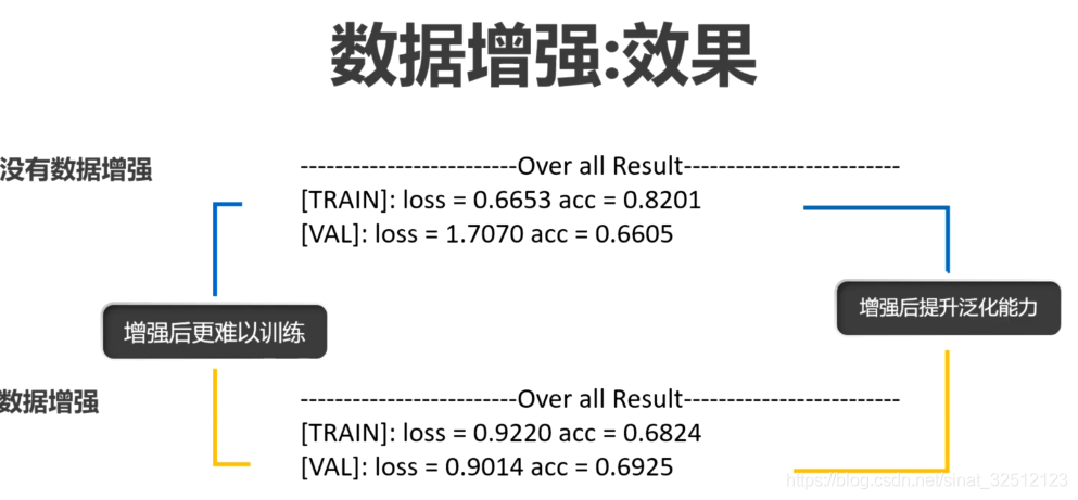
在Resnet进行训练

import numpy as np
import torch
from torch import nn
import torch.nn.functional as F
from torch.autograd import Variable
from torchvision.datasets import CIFAR10
from utils import train, resnet
from torchvision import transforms as tfs

#使用数据增强
def train_tf(x):
    im_aug=tfs.Compose([
        tfs.Resize(120),
        tfs.RandomHorizontalFlip(),
        tfs.RandomCrop(96),
        tfs.ColorJitter(brightness=0.5, contrast=0.5, hue=0.5),
        tfs.ToTensor(),
        tfs.Normalize([0.5,0.5,0.5],[0.5,0.5,0.5])
    ])
    x=im_aug(x)
    return x

def test_tf(x):
    im_aug = tfs.Compose([
        tfs.Resize(96),
        tfs.ToTensor(),
        tfs.Normalize([0.5, 0.5, 0.5], [0.5, 0.5, 0.5])
    ])
    x = im_aug(x)
    return x

train_set = CIFAR10('./data', train=True, transform=train_tf)
train_data = torch.utils.data.DataLoader(train_set, batch_size=64, shuffle=True)
test_set = CIFAR10('./data', train=False, transform=test_tf)
test_data = torch.utils.data.DataLoader(test_set, batch_size=128, shuffle=False)

net = resnet(3, 10)
optimizer = torch.optim.SGD(net.parameters(), lr=0.01)
criterion = nn.CrossEntropyLoss()
train(net, train_data, test_data, 10, optimizer, criterion)

学习率衰减

可以用torch.optim.lr_scheduler
更推荐以下这种

import numpy as np
import torch
from torch import nn
import torch.nn.functional as F
from torch.autograd import Variable
from torchvision.datasets import CIFAR10
from utils import resnet
from torchvision import transforms as tfs
from datetime import datetime
import matplotlib.pyplot as plt

#修改学习率
def set_learning_rate(optimizer, lr):
    for param_group in optimizer.param_groups:
        param_group['lr'] = lr

#使用数据增强
def train_tf(x):
    im_aug = tfs.Compose([
    tfs.Resize(120),
    tfs.RandomHorizontalFlip(),
    tfs.RandomCrop(96),
    tfs.ColorJitter(brightness=0.5, contrast=0.5, hue=0.5),
    tfs.ToTensor(),
    tfs.Normalize([0.5, 0.5, 0.5], [0.5, 0.5, 0.5])
    ])
    x = im_aug(x)
    return x
def test_tf(x):
    im_aug = tfs.Compose([
    tfs.Resize(96),
    tfs.ToTensor(),
    tfs.Normalize([0.5, 0.5, 0.5], [0.5, 0.5, 0.5])
    ])
    x = im_aug(x)
    return x

train_set = CIFAR10('./data', train=True, transform=train_tf)
train_data = torch.utils.data.DataLoader(train_set, batch_size=256, shuffle=True,num_workers=4)
valid_set = CIFAR10('./data', train=False, transform=test_tf)
valid_data = torch.utils.data.DataLoader(valid_set, batch_size=256, shuffle=False,num_workers=4)

net = resnet(3, 10)
optimizer = torch.optim.SGD(net.parameters(), lr=0.1, weight_decay=1e-4)
criterion = nn.CrossEntropyLoss()

train_losses = []
valid_losses = []

if torch.cuda.is_available():
    net=net.cuda()

prev_time = datetime.now()

for epoch in range(30):
    if epoch == 20:
        set_learning_rate(optimizer, 0.01) # 20次之后学习率修改为0.01

    net = net.train()

    train_loss = 0
    for im, label in train_data:
        if torch.cuda.is_available():
            im = Variable(im.cuda())  # (bs, 3, h, w)
            label = Variable(label.cuda())  # (bs, h, w)
        else:
            im = Variable(im)
            label = Variable(label)
        # forward
        output = net(im)
        loss = criterion(output, label)
        # backward
        optimizer.zero_grad()
        loss.backward()
        optimizer.step()

        train_loss += loss.data[0]
    cur_time = datetime.now()
    h, remainder = divmod((cur_time - prev_time).seconds, 3600)#商，余数
    m, s = divmod(remainder, 60)
    time_str = "Time %02d:%02d:%02d" % (h, m, s)

    valid_loss = 0
    valid_acc = 0
    net = net.eval()
    for im, label in valid_data:
        if torch.cuda.is_available():
            im = Variable(im.cuda(), volatile=True)#volatile功能已被移除
            label = Variable(label.cuda(), volatile=True)
        else:
            im = Variable(im, volatile=True)
            label = Variable(label, volatile=True)
            output = net(im)
        loss = criterion(output, label)
        valid_loss += loss.data[0]
        epoch_str = (
            "Epoch %d. Train Loss: %f, Valid Loss: %f, "
            % (epoch, train_loss / len(train_data), valid_loss / len(valid_data)))

        prev_time = cur_time

        train_losses.append(train_loss / len(train_data))
        valid_losses.append(valid_loss / len(valid_data))
        print(epoch_str + time_str)

#画出loss曲线
plt.plot(train_losses, label='train')
plt.plot(valid_losses, label='valid')
plt.xlabel('epoch')
plt.legend(loc='best')
"""
在第20次的时候，loss曲线陡降
"""

Dropout

正则化

optimizer = torch.optim.SGD(net.parameters(), lr=0.01, weight_decay=1e-4)

weight_decay是$\lambda$

微调进行迁移学习

fine_tuning
把一个已经很厉害的模型再微调到我们自己的数据集。

将与训练的模型导入，然后将最后的分类全连接层换成我们自己问题的全连接层，然后开始训练，
可以固定卷积层的参数，也可以不固定进行训练，最后能够非常有效地得到结果。

pytorch中内置了一些著名网络的预训练模型，模型都在torchvision.models里
比如用预训练的50层resnet，可用torchvision.models.resnet50[pretrained=True]
因为对于图片识别分类任务，最底层的卷积识别的都是一些通用的特征，比如形状、纹理等，所以对于很多图像分类、识别任务，都可以用预训练的网络得到更好的结果。

import numpy as np
import torch
from torch import nn
from torch.autograd import Variable
from torch.utils.data import DataLoader
from torchvision import models
from torchvision import transforms as tfs
from torchvision.datasets import ImageFolder
import os
from PIL import Image
import matplotlib.pyplot as plt
from utils import train

#%matplotlib inline

"""
一个数据集，二分类问题,蚂蚁和蜜蜂
"""
#可视化
root_path = './hymenoptera_data/train/'
im_list=[os.path.join(root_path,'ant',i) for i in os.listdir(root_path+'ant')[:4]]
im_list += [os.path.join(root_path, 'bees', i) for i in os.listdir(root_path +'bees')[:5]]

nrows = 3
ncols = 3
figsize = (8, 8)
_, figs = plt.subplots(nrows, ncols, figsize=figsize)

for i in range(nrows):
    for j in range(ncols):
        figs[i][j].imshow(Image.open(im_list[nrows*i+j]))
        figs[i][j].axes.get_xaxis().set_visible(False)
        figs[i][j].axes.get_yaxis().set_visible(False)
plt.show()

#定义数据预处理
train_tf = tfs.Compose([
tfs.RandomResizedCrop(224),
tfs.RandomHorizontalFlip(),
tfs.ToTensor(),
tfs.Normalize([0.485, 0.456, 0.406], [0.229, 0.224, 0.225]) # 使用ImageNet的均值和方差
])

valid_tf = tfs.Compose([
tfs.Resize(256),
tfs.CenterCrop(224),
tfs.ToTensor(),
tfs.Normalize([0.485, 0.456, 0.406], [0.229, 0.224, 0.225])
])

# 使用ImageFolder 定义数据集
train_set = ImageFolder('./hymenoptera_data/train/', train_tf)
valid_set = ImageFolder('./hymenoptera_data/val/', valid_tf)
# 使用DataLoader 定义迭代器
train_data = DataLoader(train_set, 64, True, num_workers=4)#4个线程
valid_data = DataLoader(valid_set, 128, False, num_workers=4)

#使用预训练的模型
net = models.resnet50(pretrained=True)
print(net)

#打出第一层的权重
print(net.conv1.weight)

#将最后的全连接层改为二分类
net.fc = nn.Linear(2048, 2)
criterion = nn.CrossEntropyLoss()
optimizer = torch.optim.SGD(net.parameters(), lr=1e-2, weight_decay=1e-4)
train(net, train_data, valid_data, 20, optimizer, criterion)

#可视化预测的结果
net=net.eval()#将网络改为预测模式

#读一张蚂蚁的图
im1 = Image.open('./hymenoptera_data/train/ants/0013035.jpg')
im = valid_tf(im1) # 做数据预处理
out = net(Variable(im.unsqueeze(0)).cuda())
pred_label = out.max(1)[1].data[0]#矩阵中最大的数对应的标签
print('predict label: {}'.format(train_set.classes[pred_label]))

灵活的数据读取

ImageFolder

torchvision.datasets.ImageFolder()

按照分类将同一类的放到同一个文件夹中
输入的是图片

from torchvision.datasets import ImageFolder
import torchvision.transforms as tfs

#三个文件夹，每个文件夹一个有3张图片作为例子
folder_set=ImageFolder('./example_data/image/')

#查看名称和类别下标的对应
folder_set.class_to_idx#{'class_1': 0, 'class_2': 1, 'class_3': 2}

#得到所有的图片和标签
folder_set.images
"""
[('./example_data/image/class_1/1.png', 0),
('./example_data/image/class_1/2.png', 0),
('./example_data/image/class_1/3.png', 0),
('./example_data/image/class_2/10.png', 1),
('./example_data/image/class_2/11.png', 1),
('./example_data/image/class_2/12.png', 1),
('./example_data/image/class_3/16.png', 2),
('./example_data/image/class_3/17.png', 2),
('./example_data/image/class_3/18.png', 2)]
"""

#取出其中一个数据
im,label=folder_set[0]

#传入数据预处理方式
data_tf=tfs.ToTensor()
folder_set=ImageFolder('./example_data/image/',transform=data_tf)
im,label=folder_set[0]
"""
(0 ,.,.) =
0.2314 0.1686 0.1961 ... 0.6196 0.5961 0.5804
0.0627 0.0000 0.0706 ... 0.4824 0.4667 0.4784
0.0980 0.0627 0.1922 ... 0.4627 0.4706 0.4275
... ⋱ ...
0.8157 0.7882 0.7765 ... 0.6275 0.2196 0.2078
0.7059 0.6784 0.7294 ... 0.7216 0.3804 0.3255
0.6941 0.6588 0.7020 ... 0.8471 0.5922 0.4824
(1 ,.,.) =
0.2431 0.1804 0.1882 ... 0.5176 0.4902 0.4863
0.0784 0.0000 0.0314 ... 0.3451 0.3255 0.3412
0.0941 0.0275 0.1059 ... 0.3294 0.3294 0.2863
... ⋱ ...
0.6667 0.6000 0.6314 ... 0.5216 0.1216 0.1333
0.5451 0.4824 0.5647 ... 0.5804 0.2431 0.2078
0.5647 0.5059 0.5569 ... 0.7216 0.4627 0.3608
...
[torch.FloatTensor of size 3x32x32]
"""

Dataset

输入的是txt

torch.utils.data.Dataset()

其实torchvision.datasets.ImageFolder()是torch.utils.data.Dataset()的一个子类
定义一个子类继承Dataset,重新定义__getiems__()和__len__(),前者表示按照下标取出其中一个数据，后者表示所有数据的总数。

from torch.utils.data import Dataset

#定义一个子类叫custom_dataset,继承Dataset
class custom_dataset(Dataset):
    def init__(self,txt_path,transform=None):
        self.transform=transform #传入数据预处理
        with open(txt_path,'r') as f:
            lines=f.readlines()

        self.img_list=[i.split()[0] for i in lines]
        self.label_list=[i.split()[1] for i in lines]

    def __getitem__(self,idx):#根据idx取出其中一个
        img=self.img_list[idx]
        label=self.label_list[idx]
        if self.transform is not None:
            image=self.transform(img)
        return img,label

    def __len__(self):#总数有多少
        return len(self.label_list)

txt_dataset=custom_dataset('./example_data/train.txt')#读入txt文件

#取得其中一个数据
data,label=txt_dataset[0]
print(data)
print(label)
"""
1009_2.png
YOU
"""

DataLoader

多线程迭代，batch

from torch.utils.data import DataLoader

train_data1=DataLoader(folder_set,batch_size=2,shuffle=True)#将2个数据作为一个batch
for im,label in train_data1:#访问迭代器
    print(label)
"""
1
2
[torch.LongTensor of size 2]
0
1
[torch.LongTensor of size 2]
0
2
[torch.LongTensor of size 2]
0
2
[torch.LongTensor of size 2]
1
[torch.LongTensor of size 1]
一个9个数据，有5个batch，同时打乱顺序
"""

#自定义数据
train_data2=DataLoader(txt_dataset,8,True)## batch size 设置为 8
im,label=next(iter(train_data2))#使用这种方式来访问迭代器中第一个batch的数据

collate_fn

当需要将输出的label补成相同的长短，短的用0填充，就需要使用它来自定义batch的处理方式

def collate_fn(batch):
    batch.sort(key=lambda x:len(x[1]),reverse=True )#将数据集按照label的长度从大到小排序
    img,label=zip(*batch)#将数据和label配对取出
    #填充
    pad_label=[]
    lens=[]
    max_len=len(label[0])
    for i in range(len(label)):
        temp_label=label[i]
        temp_label+='0'*(max_len-len(label[i]))
        pad_label.append(temp_label)
        lens.append(len(label[i]))
    return img,pad_label,lens#输出label的真实长度

train_data3=DataLoader(txt_dataset,8,True,collate_fn=collate_fn)
img,label,lens=next(iter(train_data3))

批标准化

BN详解

import torch

def simple_batch_norm_1d(x,gamma,beta):
    eps=1e-5
    x_mean=torch.mean(x,dim=0,keepdim=True)#列向量，保留维度进行broadcast,均值
    x_var=torch.mean((x-x_mean)**2,dim=0,keepdim=True)
    x_var=torch.sqrt(x_var+eps)#标准差
    x_hat=(x-x_mean)/x_var
    return gamma.view_as(x_mean)*x_hat+beta.vie_as(x_mean)#将gamma,beta变为和均值一个大小

#验证对于任意输入，输出是否能标准化
x=torch.arange(15).view(5,3)
gamma=torch.ones(x.shape[1])
beta=torch.ones(x.shape[1])
print('before bn: ')
print(x)
y=simple_batch_norm_1d(x,gamma,beta)
print('after bn: ')
print(y)
"""
before bn:
0 1 2
3 4 5
6 7 8
9 10 11
12 13 14
[torch.FloatTensor of size 5x3]

after bn:
-1.4142 -1.4142 -1.4142
-0.7071 -0.7071 -0.7071
0.0000 0.0000 0.0000
0.7071 0.7071 0.7071
1.4142 1.4142 1.4142
[torch.FloatTensor of size 5x3]
5个数据点，三个特征，每一列表示一个特征 的不同数据点
"""

测试的适合该使用批标准化，否则会导致结果出现偏差。
测试的时候不能用测试的数据集去算均值和方差，而是用训练时算出的移动平均均值和方差去代替
用一下能区分训练状态和测试状态的批标准化方法

import torch
from torch import nn

def batch_norm_1d(x, gamma, beta, is_training, moving_mean, moving_var,moving_momentum=0.1):
    eps=1e-5
    x_mean=torch.means(x,dim=0,keepdim=True)#保留维度进行broadcast
    x_var=torch.means((x-x_mean)**2,dim=0,keepdim=True)
    if is_training:
        x_hat = (x - x_mean) / torch.sqrt(x_var + eps)
        moving_mean[:]=moving_momentum*moving_mean+(1.-moving_momentum)*x_mean
        moving_var[:] = moving_momentum * moving_var + (1. - moving_momentum) * x_var
    else:
        x_hat = (x - moving_mean) / torch.sqrt(moving_var + eps)
    return gamma.view_as(x_mean) * x_hat + beta.view_as(x_mean)

pytorch实现

使用批标准化的情况能够更快地收敛。
mnist数据集

import torch
import numpy as np
from torchvision.datasets import mnist # 导入pytorch内置的mnist
from torch.utils.data import DataLoader
from torch import nn
from torch.autograd import Variable
from utils import train

def batch_norm_1d(x, gamma, beta, is_training, moving_mean, moving_var,moving_momentum=0.1):
    eps=1e-5
    x_mean=torch.means(x,dim=0,keepdim=True)#保留维度进行broadcast
    x_var=torch.means((x-x_mean)**2,dim=0,keepdim=True)
    if is_training:
        x_hat = (x - x_mean) / torch.sqrt(x_var + eps)
        moving_mean[:]=moving_momentum*moving_mean+(1.-moving_momentum)*x_mean
        moving_var[:] = moving_momentum * moving_var + (1. - moving_momentum) * x_var
    else:
        x_hat = (x - moving_mean) / torch.sqrt(moving_var + eps)
    return gamma.view_as(x_mean) * x_hat + beta.view_as(x_mean)

def data_tf(x):
    x = np.array(x, dtype='float32') / 255
    x = (x - 0.5) / 0.5 #
    x = x.reshape((-1,)) #拉平
    x = torch.from_numpy(x)
    return x

#使用内置函数下载mnist数据集
train_set = mnist.MNIST('./data', train=True, transform=data_tf, download=True)
test_set = mnist.MNIST('./data', train=False, transform=data_tf, download=True)
train_data = DataLoader(train_set, batch_size=64, shuffle=True)
test_data = DataLoader(test_set, batch_size=128, shuffle=False)

class multi_network(nn.Module):
    def __init__(self):
        super(multi_network, self).__init__()
        self.layer1 = nn.Linear(784, 100)
        self.relu = nn.ReLU(True)
        self.layer2 = nn.Linear(100, 10)

        self.gamma=nn.Parameter(torch.randn(100))
        self.beta = nn.Parameter(torch.randn(100))

        self.moving_mean = Variable(torch.zeros(100))
        self.moving_var = Variable(torch.zeros(100))

    def forward(self, x, is_train=True):
        x = self.layer1(x)
        x = batch_norm_1d(x, self.gamma, self.beta, is_train, self.moving_mean,self.moving_var)
        x = self.relu(x)
        x = self.layer2(x)
        return x


net=multi_network()
criterion = nn.CrossEntropyLoss()
optimizer = torch.optim.SGD(net.parameters(), 1e-1)
train(net, train_data, test_data, 10, optimizer, criterion)

"""
gamma和beta可以作为参数进行训练，初始化为随机的高斯分布
moving_mean和moving_var都初始化为0，并不是更新的参数，训练完后，它们的值会变
"""
print(net.moving_mean[:10])
"""
Variable containing:
0.5505
2.0835
0.0794
-0.1991
-0.9822
-0.5820
0.6991
-0.1292
2.9608
1.0826
[torch.FloatTensor of size 10]
"""

还可以有内置函数torch.nn.BatchNorm1d()和torch.nn.BatchNorm2d()，pytorch中将gamma、beta、moving_mean和moving_var都作为参数进行训练。

TensorBoard可视化

是tensorflow中非常好用的可视化工具
pytorch中也可以用。

安装 tensorflow 和 tensorboardX

pip install tensorflow
pip install tensorboradX

画计算图不大支持，但可以画出loss曲线

import numpy as np
import torch
from torch import nn
import torch.nn.functional as F
from torch.autograd import Variable
from torchvision.datasets import CIFAR10
from utils import resnet
from torchvision import transforms as tfs
from datetime import datetime
from tensorboardX import SummaryWriter

#使用数据增强
def train_tf(x):
    im_aug = tfs.Compose([
    tfs.Resize(120),
    tfs.RandomHorizontalFlip(),
    tfs.RandomCrop(96),
    tfs.ColorJitter(brightness=0.5, contrast=0.5, hue=0.5),
    tfs.ToTensor(),
    tfs.Normalize([0.5, 0.5, 0.5], [0.5, 0.5, 0.5])
    ])
    x = im_aug(x)
    return x

def test_tf(x):
    im_aug = tfs.Compose([
    tfs.Resize(96),
    tfs.ToTensor(),
    tfs.Normalize([0.5, 0.5, 0.5], [0.5, 0.5, 0.5])
    ])
    x = im_aug(x)
    return x

train_set = CIFAR10('./data', train=True, transform=train_tf)
train_data = torch.utils.data.DataLoader(train_set, batch_size=256, shuffle=True,num_workers=4)
valid_set = CIFAR10('./data', train=False, transform=test_tf)
valid_data = torch.utils.data.DataLoader(valid_set, batch_size=256, shuffle=False,num_workers=4)

net = resnet(3, 10)
optimizer = torch.optim.SGD(net.parameters(), lr=0.1, weight_decay=1e-4)
criterion = nn.CrossEntropyLoss()

writer=SummaryWriter()

def get_acc(output,label):
    total=output.shape[0]
    _,pred_label=output.max(1)
    num_correct=(pred_label==label).sum().data[0]
    return num_correct/total

if torch.cuda.is_available():
    net=net.cuda()

prev_time=datetime.now()

for epoch in range(30):
    train_loss=0
    train_acc=0
    net=net.train()
    for im,label in train_data:
        if torch.cuda.is_available():
            im=Variable(im.cuda())## (bs, 3, h, w)
            label=Variable(label.cuda())#(bs,h,w)
        else:
            im = Variable(im)  ## (bs, 3, h, w)
            label = Variable(label)  # (bs,h,w)
        #forward
        out=net(im)
        loss=criterion(out,label)
        #backward
        optimizer.zero_grad()
        loss.backward()
        optimizer.step()

        train_loss+=loss.data[0]
        train_acc+=get_acc(out,label)

    cur_time=datetime.now()
    h, remainder = divmod((cur_time - prev_time).seconds, 3600)
    m, s = divmod(remainder, 60)
    time_str = "Time %02d:%02d:%02d" % (h, m, s)

    valid_loss = 0
    valid_acc = 0
    net = net.eval()
    for im, label in valid_data:
        if torch.cuda.is_available():
            im = Variable(im.cuda(), volatile=True)
            label = Variable(label.cuda(), volatile=True)
        else:
            im = Variable(im, volatile=True)
            label = Variable(label, volatile=True)
        output = net(im)
        loss = criterion(output, label)
        valid_loss += loss.data[0]
        valid_acc += get_acc(output, label)

    epoch_str = ("Epoch %d. Train Loss: %f, Train Acc: %f, Valid Loss: %f, Valid Acc:%f, "
                 % (epoch, train_loss / len(train_data),train_acc / len(train_data), valid_loss / len(valid_data),
                    valid_acc / len(valid_data)))
    prev_time = cur_time



#========================使用tensorboard===============================
writer.add_scalars('Loss',{'train':train_loss/len(train_data),
                           'valid':valid_loss/len(valid_data)},epoch)

writer.add_scalars('acc',{'train':train_acc/len(train_data),
                           'valid':valid_acc/len(valid_data)},epoch)
#========================================================================
print(epoch_str+time_str)

训练完成后，目录中会出现一个文件夹叫runs,在终端运行

tensorboard --logdir runs