【译：scikit learn学习】有监督的神经网络模型Neural network models (supervised)

最新推荐文章于 2024-08-10 01:22:01 发布

sinat_33400946

最新推荐文章于 2024-08-10 01:22:01 发布

阅读量5k

点赞数

分类专栏：机器学习文章标签：神经网络

机器学习专栏收录该内容

1 篇文章 0 订阅

订阅专栏

本文介绍了scikit-learn中的多层感知器（MLP）模型，这是一种有监督学习算法，适用于非线性回归和分类任务。MLP包含至少一个隐藏层，其损失函数可能具有局部极小值，需要调整参数以避免过拟合。文章还讨论了其在线学习、分类、回归和正则化的特点，并提供了不同学习策略和正则化效果的示例。

摘要由CSDN通过智能技术生成

参考：http://scikit-learn.org/stable/modules/neural_networks_supervised.html#neural-networks-supervised

Multi-layer Perceptron 多层感知器

Multi-layer Perceptron (MLP)多层感知器是有监督的学习算法，通过训练数据集，学习得到函数 $f(\cdot): R^m \rightarrow R^o$ ，其中m是输入的维数，o是输出的维数。给定一组特征值 $X = {x_1, x_2, ..., x_m}$ ，以及目标值 $y$ ，它可以学习训练出一非线性函数用于近似回归或者分类。它不同于逻辑回归，在输入层与输出层之间，可能会有一个或多个非线性层，我们把它称作隐层。下图展示了单隐层的具有标量输出的多层感知器。

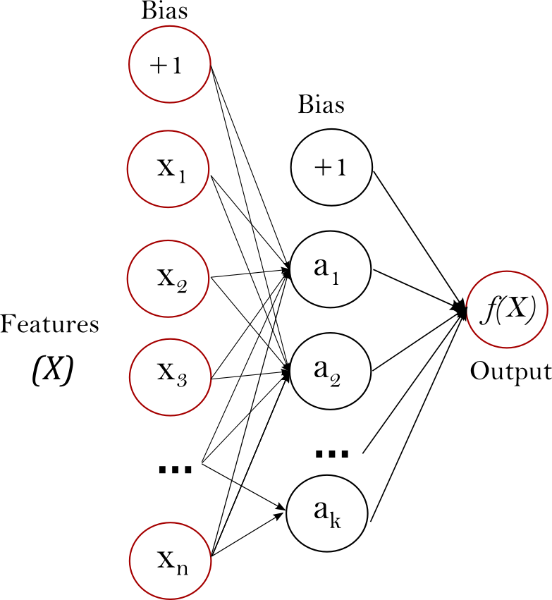
Figure 1 : One hidden layer MLP.

最左边的就是输入层，包含一组神经元 $\{x_i | x_1, x_2, ..., x_m\}$ ，以代表输入特征。隐层中的神经元将前一层的值，通过加权的线性计算公式 $w_1x_1 + w_2x_2 + ... + w_mx_m$ 进行传值，紧跟着激活函数 $g(\cdot):R \rightarrow R$ ，比如双曲线正切函数。输出层接收到最后一层隐层传来的值后转换为输出值。

模型包含共同的特征coefs_ 和intercepts_. 。coefs_是一列权值矩阵，在i 处的权值矩阵代表i层与i+1层之间的权值。intercepts_是权值矩阵偏差向量，在i处的向量代表增加到i+1层的偏差值。

多层感知器的优势是：

能够学习非线性模型

能够使用partial_fit实时在线学习模型

多层感知器的缺点包括如下：

具有隐层的多层感知器有非凸损失函数，存在局部极小值。因此不同的随机权值初始化可能导致不同的验证精度。

多层感知器需要调整一些参数，如隐层神经元数量，层数和迭代次数等

多层感知器对特征缩放敏感

Please see Tips on Practical Use section that addresses some of these disadvantages.

Classification 分类

类 MLPClassifier 实现了多层感知算法（MLP），使用 Backpropagation 训练。

MLP训练两组数组：array X of size (n_samples, n_features)，其包含表示为浮点特征向量的训练样本。array y of size (n_samples,)，包含训练样本的目标值。

>>> from sklearn.neural_network import MLPClassifier
>>> X = [[0., 0.], [1., 1.]]
>>> y = [0, 1]
>>> clf = MLPClassifier(solver='lbfgs', alpha=1e-5,
...                     hidden_layer_sizes=(5, 2), random_state=1)
...
>>> clf.fit(X, y)                         
MLPClassifier(activation='relu', alpha=1e-05, batch_size='auto',
       beta_1=0.9, beta_2=0.999, early_stopping=False,
       epsilon=1e-08, hidden_layer_sizes=(5, 2), learning_rate='constant',
       learning_rate_init=0.001, max_iter=200, momentum=0.9,
       nesterovs_momentum=True, power_t=0.5, random_state=1, shuffle=True,
       solver='lbfgs', tol=0.0001, validation_fraction=0.1, verbose=False,
       warm_start=False)

经过训练之后的模型即可为新的样本预测分类

>>> clf.predict([[2., 2.], [-1., -2.]])
array([1, 0])

MLP可以进行非线性模型的训练。clf.coefs_ 包含权值矩阵

>>> [coef.shape for coef in clf.coefs_]
[(2, 5), (5, 2), (2, 1)]

MLPClassifier s只支持交叉熵损失函数。通过使用predict_proba 方法可以概率估计。

MLP使用反向传播Backpropagation进行训练。为了更精确，训练使用梯度下降，且梯度使用反向传播算法Backpropagation计算。对于分类，其最小化了交叉熵损失函数，通过给出每个样本x的概率估计 $P(y|x)$ 的向量：

>>> clf.predict_proba([[2., 2.], [1., 2.]])  
array([[  1.967...e-04,   9.998...-01],
       [  1.967...e-04,   9.998...-01]])

MLPClassifier 支持多类别分类，是使用Softmax作为输出函数。

the model supports multi-label classification in which a sample can belong to more than one class. For each class, the raw output passes through the logistic function. Values larger or equal to 0.5 are rounded to 1, otherwise to 0. For a predicted output of a sample, the indices where the value is 1 represents the assigned classes of that sample:

除此之外，模型支持多标签分类 multi-label classification除，即一个样本可能属于不知一个类。对于每一个类，原始输出通过logistic 函数。值大于或等于0.5判为1，否则等于0。一个样本的预测输出，值是1 的参数代表指定为样本的类。

>>> X = [[0., 0.], [1., 1.]]
>>> y = [[0, 1], [1, 1]]
>>> clf = MLPClassifier(solver='lbfgs', alpha=1e-5,
...                     hidden_layer_sizes=(15,), random_state=1)
...
>>> clf.fit(X, y)                         
MLPClassifier(activation='relu', alpha=1e-05, batch_size='auto',
       beta_1=0.9, beta_2=0.999, early_stopping=False,
       epsilon=1e-08, hidden_layer_sizes=(15,), learning_rate='constant',
       learning_rate_init=0.001, max_iter=200, momentum=0.9,
       nesterovs_momentum=True, power_t=0.5, random_state=1, shuffle=True,
       solver='lbfgs', tol=0.0001, validation_fraction=0.1, verbose=False,
       warm_start=False)
>>> clf.predict([[1., 2.]])
array([[1, 1]])
>>> clf.predict([[0., 0.]])
array([[0, 1]])

See the examples below and the doc string of MLPClassifier.fit for further information

Examples:

Regression 回归

类 MLPRegressor 通过输出层没有激活函数的反向传播算法，或者也可看做恒等函数作为激活函数，实现了多层感知器。因此，其使用方差作为损失函数，输出是利系列连续的值。

MLPRegressor 也支持多输出的回归，即一个样本可能有不止一个目标值。

Regularization

Both MLPRegressor and class: MLPClassifier use parameter alpha for regularization (L2 regularization) term which helps in avoiding overfitting by penalizing weights with large magnitudes. Following plot displays varying decision function with value of alpha.

MLPRegressor 和类：MLPClassifier都使用了参数alpha 用于正则化 (L2 regularization)，通过大幅度的惩罚权重防止过拟合。下图显示不同的alpha值的判定函数

../_images/sphx_glr_plot_mlp_alpha_0011.png

See the examples below for further inform

Examples:

Varying regularization in Multi-layer Perceptron

Algorithms 算法

MLP trains using Stochastic Gradient Descent , Adam , or L-BFGS . Stochastic Gradient Descent (SGD) updates parameters using the gradient of the loss function with respect to a parameter that needs adaptation, i.e.
MLP使用随机梯度下降，Adam，或者L-BFGS。GSD使用参照需要调整参数的损失函数的梯度来更新参数。i.e.

$w \leftarrow w - \eta (\alpha \frac{\partial R(w)}{\partial w}+ \frac{\partial Loss}{\partial w})$