# [cs231n （八）神经网络总结：最小网络案例研究 ][1]

cs231n （八）神经网络总结：最小网络案例研究

标签（空格分隔）： 神经网络

同类文章

cs231n （一）图像分类识别讲了KNN
cs231n （二）讲了线性分类器：SVM和SoftMax
cs231n （三）优化问题及方法
cs231n （四）反向传播
cs231n （五）神经网络 part 1:构建架构
cs231n （六）神经网络 part 2:传入数据和损失
cs231n （七）神经网络 part 3 : 学习和评估
cs231n （八）神经网络总结：最小网络案例研究
cs231n （九）卷积神经网络

---

0.回顾

cs231n （一）图像分类识别讲了KNN
cs231n （二）讲了线性分类器：SVM和SoftMax
cs231n （三）优化问题及方法
cs231n （四）反向传播
cs231n （五）神经网络 part 1:构建架构
cs231n （六）神经网络 part 2:传入数据和损失
cs231n （七）神经网络 part 3 : 学习和评估

1. 引言

经过前面近七节课的学习训练，我们有了深厚理论基础，和毛毛草草的向量化编程基础、调优基础。。。这牛逼吹的怕了都。

那么现在我们应该开始自己动手解决一个实际问题吧：快来啊。

首先实现线性分类器，然后拓展到神经网络，只要线性网络构建好了，我们拓展到神经网络就会很简单很简单很jian。

2. 生成一些数据

先生成一个螺旋离散数据

N = 100 # number of points per class
D = 2 # dimensionality
K = 3 # number of classes
X = np.zeros((N*K,D)) # data matrix (each row = single example)
y = np.zeros(N*K, dtype='uint8') # class labels
for j in range(K):
  ix = range(N*j,N*(j+1))
  r = np.linspace(0.0,1,N) # radius
  t = np.linspace(j*4,(j+1)*4,N) + np.random.randn(N)*0.2 # theta
  X[ix] = np.c_[r*np.sin(t), r*np.cos(t)]
  y[ix] = j
# lets visualize the data:
plt.scatter(X[:, 0], X[:, 1], c=y, s=40, cmap=plt.cm.Spectral)
plt.show()

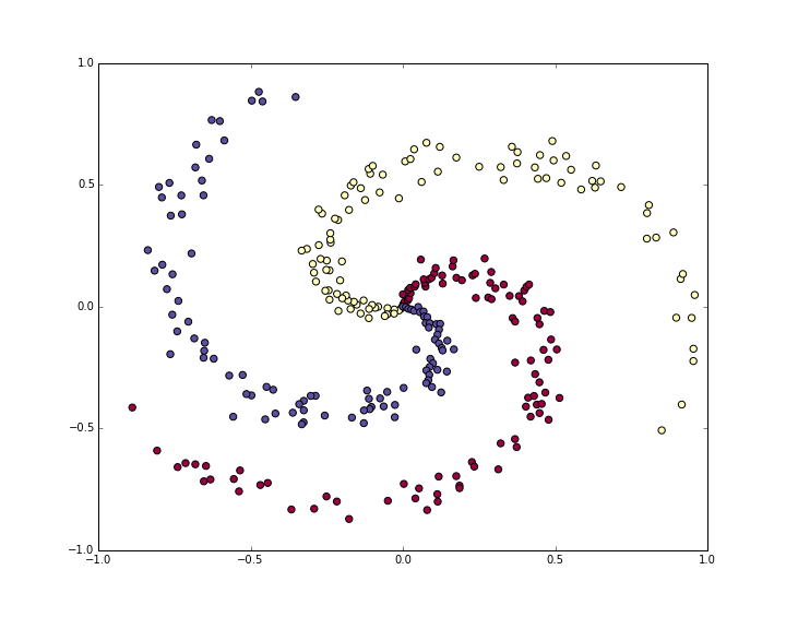
此时数据是非线性的， 对数据进行标准差标准化已经做过了。

3. 训练一个softmax线性分类器

1. 初始化参数

先在这个分类数据集上训练一个Softmax分类器，Softmax分类器具有线性分数函数，并使用交叉熵损失。

线性分类器的参数由每个类别的权重矩阵W和偏差矢量b组成，先将这些参数初始化为随机数：

# initialize parameters randomly
W = 0.01 * np.random.randn(D,K)
b = np.zeros((1,K))

W = DxC = 2x3

2. 计算分数

得到分数很简答啊：

# compute class scores for a linear classifier
scores = np.dot(X, W) + b

X = NxD = 300x2
scores = NxC

3. 计算loss

损失函数是得到区分目标的关键：其实就是正确的类得分是最高的，并且损失是最低的，如果分类正确。

这里使用的是softmax相关的交叉熵损失，损失函数应该是：

$$Li=-log(\frac{e^{f_{y_i}}}{{\sum }_j{e}^{f_j}})$$

softmax 函数把每一个数据得到三个分数，按照上述公式得到的是标准化概率，并且：
当正确类别概率很小，那么loss会趋近于无穷的。
当正确类别概率接近于1，那么loss会趋近于0的， 因为log(1)=0

$$L = \underbrace{ \frac{1}{N} \sum_i L_i }\text{data loss} + \underbrace{ \frac{1}{2} \lambda \sum_k\sum_l W{k,l}^2 }_\text{regularization loss} \\$$

我们计算得到了分数，那么损失可由上述狮子计算

num_examples = X.shape[0]
# get unnormalized probabilities
exp_scores = np.exp(scores)
# normalize them for each example
probs = exp_scores / np.sum(exp_scores, axis=1, keepdims=True)

现在得到的概率是：[300 x 3], 每行有三个数值，理论上最大的那个就是对应的正确分类的分数。

corect_logprobs = -np.log(probs[range(num_examples),y])

这里只分配概率给正确分类，损失就是这些对数概率和正则化损失的均值

# compute the loss: average cross-entropy loss and regularization
data_loss = np.sum(corect_logprobs)/num_examples
reg_loss = 0.5*reg*np.sum(W*W)
loss = data_loss + reg_loss

损失越低意味着正确分类的概率越高。

4. 反向传播法计算梯度

这里引入 $p_k=\frac{e^{f_k}}{{\sum }_j{e}^{f_j}}{L}_i=-\log \left(p_{y_i}\right)$,

可以使用链式法则：

$$\frac{\partial L_i}{\partial f_k}=p_k-1(y_i=k)$$

好简单哈 p = [0.2, 0.3, 0.5], 0.3是正确的分类， 那么 df = [0.2, -0.7, 0.5]

增加分数向量f的第一个或最后一个元素（不正确类别的分数）会增加损失（由于+0.2和+0.5的正号）增加损失是不好的分类。

然而，增加正确分数的分数对损失有负面影响。 -0.7的梯度告诉我们，增加正确的分数会导致损失 Li 的减少，这是合理的。

probs存储每个例子的所有类（作为行）的概率，为了获得分数上的梯度dscores。

dscores = probs
dscores[range(num_examples),y] -= 1
dscores /= num_examples

最后，我们得到的分数 $scores=np.dot（X，W）+b$ ，所以分数梯度保存在dscores中），我们现在可以反向传播到W和b：

dW = np.dot(X.T, dscores)
db = np.sum(dscores, axis=0, keepdims=True)
dW += reg*W # don't forget the regularization gradient

###5. 如何参数更新？

现在指导了梯度，指导参数如何影响损失函数，那么就开始更新梯度啦，就是稍微减少点梯度，其实就是迭代啦。

# perform a parameter update
W += -step_size * dW
b += -step_size * db

6. 现在就可以合并一下得到softmax分类器

#Train a Linear Classifier

# initialize parameters randomly
W = 0.01 * np.random.randn(D,K)
b = np.zeros((1,K))

# some hyperparameters
step_size = 1e-0
reg = 1e-3 # regularization strength

# gradient descent loop
num_examples = X.shape[0]
for i in xrange(200):
  
  # evaluate class scores, [N x K]
  scores = np.dot(X, W) + b 
  
  # compute the class probabilities
  exp_scores = np.exp(scores)
  probs = exp_scores / np.sum(exp_scores, axis=1, keepdims=True) # [N x K]
  
  # compute the loss: average cross-entropy loss and regularization
  corect_logprobs = -np.log(probs[range(num_examples),y])
  data_loss = np.sum(corect_logprobs)/num_examples
  reg_loss = 0.5*reg*np.sum(W*W)
  loss = data_loss + reg_loss
  if i % 10 == 0:
    print "iteration %d: loss %f" % (i, loss)
  
  # compute the gradient on scores
  dscores = probs
  dscores[range(num_examples),y] -= 1
  dscores /= num_examples
  
  # backpropate the gradient to the parameters (W,b)
  dW = np.dot(X.T, dscores)
  db = np.sum(dscores, axis=0, keepdims=True)
  
  dW += reg*W # regularization gradient
  
  # perform a parameter update
  W += -step_size * dW
  b += -step_size * db

结果大概是这个样子的。

iteration 0: loss 1.096956
iteration 10: loss 0.917265
iteration 20: loss 0.851503
iteration 30: loss 0.822336
iteration 40: loss 0.807586
iteration 50: loss 0.799448
iteration 60: loss 0.794681
iteration 70: loss 0.791764
iteration 80: loss 0.789920
iteration 90: loss 0.788726
iteration 100: loss 0.787938
iteration 110: loss 0.787409
iteration 120: loss 0.787049
iteration 130: loss 0.786803
iteration 140: loss 0.786633
iteration 150: loss 0.786514
iteration 160: loss 0.786431
iteration 170: loss 0.786373
iteration 180: loss 0.786331
iteration 190: loss 0.786302

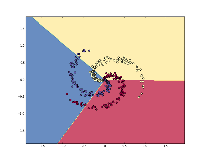
经过190次迭代，可以得到训练精度：

# evaluate training set accuracy
scores = np.dot(X, W) + b
predicted_class = np.argmax(scores, axis=1)
print 'training accuracy: %.2f' % (np.mean(predicted_class == y))

准确率是 49%， 看一下学习到边界

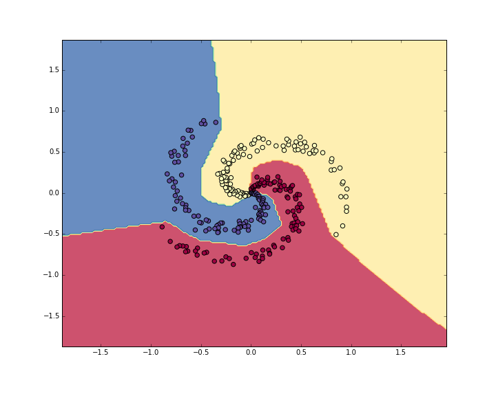
4. 训练神经网络

其实对于非线性边界用线性分类器确实有点难，现在我们构建一个简单的二层神经网络。

第一层第二层就是这么简单：

# initialize parameters randomly
h = 100 # size of hidden layer
W = 0.01 * np.random.randn(D,h)
b = np.zeros((1,h))
W2 = 0.01 * np.random.randn(h,K)
b2 = np.zeros((1,K))

前向传播的分数可以这样得到：

# evaluate class scores with a 2-layer Neural Network
hidden_layer = np.maximum(0, np.dot(X, W) + b) # note, ReLU activation
scores = np.dot(hidden_layer, W2) + b2

在隐含层添加非线性单元------ReLU。
然后计算loss，分数梯度dscores都和之前一样。
计算梯度的时候先BP到第二层网络，这里也和之前的softmax类似。

# backpropate the gradient to the parameters
# first backprop into parameters W2 and b2
dW2 = np.dot(hidden_layer.T, dscores)
db2 = np.sum(dscores, axis=0, keepdims=True)

由于中间加了一个隐含层，所以我们需要计算隐含层的梯度：

dhidden = np.dot(dscores, W2.T)

还需要回传ReLUd的非线性，很简答啊
$r=max(0,x),\frac{dr}{dx}=1(x>0)$
可以知道梯度通过如果x > 0， 梯度为零如果x < 0

# backprop the ReLU non-linearity
dhidden[hidden_layer <= 0] = 0

那么计算第一层的权重和梯度就是：

# finally into W,b
dW = np.dot(X.T, dhidden)
db = np.sum(dhidden, axis=0, keepdims=True)

好了我们已经完成整个过程了，总结一下。

# initialize parameters randomly
h = 100 # size of hidden layer
W = 0.01 * np.random.randn(D,h)
b = np.zeros((1,h))
W2 = 0.01 * np.random.randn(h,K)
b2 = np.zeros((1,K))

# some hyperparameters
step_size = 1e-0
reg = 1e-3 # regularization strength

# gradient descent loop
num_examples = X.shape[0]
for i in xrange(10000):
  
  # evaluate class scores, [N x K]
  hidden_layer = np.maximum(0, np.dot(X, W) + b) # note, ReLU activation
  scores = np.dot(hidden_layer, W2) + b2
  
  # compute the class probabilities
  exp_scores = np.exp(scores)
  probs = exp_scores / np.sum(exp_scores, axis=1, keepdims=True) # [N x K]
  
  # compute the loss: average cross-entropy loss and regularization
  corect_logprobs = -np.log(probs[range(num_examples),y])
  data_loss = np.sum(corect_logprobs)/num_examples
  reg_loss = 0.5*reg*np.sum(W*W) + 0.5*reg*np.sum(W2*W2)
  loss = data_loss + reg_loss
  if i % 1000 == 0:
    print "iteration %d: loss %f" % (i, loss)
  
  # compute the gradient on scores
  dscores = probs
  dscores[range(num_examples),y] -= 1
  dscores /= num_examples
  
  # backpropate the gradient to the parameters
  # first backprop into parameters W2 and b2
  dW2 = np.dot(hidden_layer.T, dscores)
  db2 = np.sum(dscores, axis=0, keepdims=True)
  # next backprop into hidden layer
  dhidden = np.dot(dscores, W2.T)
  # backprop the ReLU non-linearity
  dhidden[hidden_layer <= 0] = 0
  # finally into W,b
  dW = np.dot(X.T, dhidden)
  db = np.sum(dhidden, axis=0, keepdims=True)
  
  # add regularization gradient contribution
  dW2 += reg * W2
  dW += reg * W
  
  # perform a parameter update
  W += -step_size * dW
  b += -step_size * db
  W2 += -step_size * dW2
  b2 += -step_size * db2
  
  
## This prints:

iteration 0: loss 1.098744
iteration 1000: loss 0.294946
iteration 2000: loss 0.259301
iteration 3000: loss 0.248310
iteration 4000: loss 0.246170
iteration 5000: loss 0.245649
iteration 6000: loss 0.245491
iteration 7000: loss 0.245400
iteration 8000: loss 0.245335
iteration 9000: loss 0.245292

训练精度是：98%! 厉害了，老铁

# evaluate training set accuracy
hidden_layer = np.maximum(0, np.dot(X, W) + b)
scores = np.dot(hidden_layer, W2) + b2
predicted_class = np.argmax(scores, axis=1)
print 'training accuracy: %.2f' % (np.mean(predicted_class == y))

5. 总结

其实从线性到网络我们变化的代码很少，Loss只变了一行，反向传播只不过是加了“中间变量”。

---

转载和疑问声明

如果你有什么疑问或者想要转载，没有允许是不能转载的哈
赞赏一下能不能转？哈哈，联系我啊，我告诉你呢 ~~
欢迎联系我哈，我会给大家慢慢解答啦~~~怎么联系我？ 笨啊~ ~~ 你留言也行

你关注微信公众号1.机器学习算法工程师：2.或者扫那个二维码，后台发送 “我要找朕”，联系我也行啦！

（爱心.gif） 么么哒 ~么么哒 ~么么哒
码字不易啊啊啊，如果你觉得本文有帮助，三毛也是爱！

我祝各位帅哥，和美女，你们永远十八岁，嗨嘿嘿~~~