Convolutional Neural Networks for Sentence Classification-经典论文复现活动(MindSpore)

This article focuses on implementing sentence-level classification tasks with convolutional neural networks (CNNs). These networks are trained using pre-trained word vectors, and the implementation is conducted using the MindSpore AI framework. 

Main Task 

任务描述 

参考任务清单中paperswithcode链接，学习论文中的网络模型，基于MindSpore框架完成对应网络模型的复现。任务要求 

1. 建议基于MindSpore框架最新版本（Nightly）进行开发，不能使用其他AI框架的接口。最新版本安装请参考：https://www.mindspore.cn/install 选择Nightly版本。 

2. 任务分为两部分： 

1. ①【推理】完成网络模型和权重转成MindSpore格式并做推理； 
2. ②【训练】在完成推理之后，需要完成从0到1的训练； 

3. 代码提交至个人github开源仓库，并在paperswithcode网站对应的论文下添加自己的代码实现。 

4. 代码完成之后，在昇思MindSpore论坛、CSDN、知乎等任一平台发帖分享自己的项目实现过程与经验。 

Overview 

Conventionally, Convolutional Neural Networks (CNNs) are deployed for image analysis. They typically comprise one or more convolutional layers, followed by one or more linear layers. The convolutional layers utilize filters (also known as kernels or receptive fields), which scan over an image, yielding a processed version. This processed image can then be passed into another convolutional layer or a linear layer. Each filter possesses a specific shape, such as a 3x3 filter spanning a 3-pixel wide and high area of the image, with every element of the filter assigned a specific weight. While these weights were manually set by engineers in traditional image processing, the key advantage of convolutional layers in neural networks is that these weights are learned via backpropagation. 

The concept underlying the learning of weights is that convolutional layers function as feature extractors, pinpointing key components of the image significant for the CNN's objective. For example, if a CNN is used for face detection in images, it might seek features like the presence of a nose, mouth, or eyes. 

However, why apply CNNs to text? Similarly to how a 3x3 filter scans a patch of an image, a 1x2 filter can traverse two sequential words in a piece of text (a bi-gram). In our previous discussion, we considered the FastText model that employed bi-grams by explicitly appending them to the end of a text. However, in this CNN model, we will use various filter sizes to examine bi-grams (using a 1x2 filter), tri-grams (a 1x3 filter), or n-grams (a 1x n filter) within the text. 

The fundamental idea is that the presence of certain bi-grams, tri-grams, and n-grams in a review will provide insightful indicators of the final sentiment. 

Environment 

To meet the requirement of using the MindSpore Nightly version, you can easily download it using the command pip install mindspore-dev -i https://pypi.tuna.tsinghua.edu.cn/simple. This will install the development version of MindSpore, incorporating the latest features and updates. By utilizing the Tsinghua mirror, you can ensure efficient and reliable downloads. 

For the implementation, I have decided to utilize the mindspore_2.0_train image. This image provides a preconfigured environment specifically designed for training tasks using MindSpore version 2.0. It includes all the necessary tools and libraries to effectively work with MindSpore 

​

Data preparation 

Dataset 

This paper utilizes the IMDB movie review dataset, a renowned collection frequently employed for tasks related to sentence-level classification tasks.. The dataset is composed of two classifications: Positive and Negative. Below is an illustration: 

Review	Label
This movie is an absolute gem! The acting is superb, the storyline is gripping, and the cinematography is breathtaking. I was completely engrossed from start to finish. The characters are well-developed, and I found myself emotionally invested in their journeys. The dialogue is witty and thought-provoking, and the pacing is perfect. The director has truly created a masterpiece that will stand the test of time. I cannot recommend this film highly enough. It's a must-see for any cinema lover!	Positive
I had high expectations for this movie, but it turned out to be a major letdown. The acting was wooden, and the performances felt forced. The plot was convoluted and lacked coherence, leaving me confused and unsatisfied. The editing was choppy, making it difficult to follow the story. Additionally, the dialogue was clichéd and uninspiring. The whole experience felt like a waste of time and money. I wouldn't recommend this movie to anyone. Save yourself the disappointment and skip it.	Negative

The IMDB dataset I've acquired is in the format of a tar.gz file. To read and extract the information from it, I employ the Python tarfile library, separating and storing all the data and labels independently. Here's how the original IMDB dataset directory looks after decompression: 

├── aclImdb 
│   ├── imdbEr.txt 
│   ├── imdb.vocab 
│   ├── README 
│   ├── test 
│   └── train 
│         ├── neg 
│         ├── pos 复制

The dataset is bifurcated into two sections, namely 'train' and 'test'. Each of these sections further contains two folders labeled 'neg' and 'pos'. Hence, the 'train' and 'test' data, along with their respective labels, need to be individually read and processed. 

import re 
import six 
import string 
import tarfile 
 
class IMDBData(): 
    label_map = { 
        "pos": 1, 
        "neg": 0 
    } 
    def __init__(self, path, mode="train"): 
        self.mode = mode 
        self.path = path 
        self.docs, self.labels = [], [] 
        self._load("pos") 
        self._load("neg") 
    def _load(self, label): 
        pattern = re.compile(r"aclImdb/{}/{}/.*\.txt$".format(self.mode, label)) 
        with tarfile.open(self.path) as tarf: 
            tf = tarf.next() 
            while tf is not None: 
                if bool(pattern.match(tf.name)): 
               self.docs.append(str(tarf.extractfile(tf).read().rstrip(six.b("\n\r")) 
                                         .translate(None, six.b(string.punctuation)).lower()).split()) 
                    self.labels.append([self.label_map[label]]) 
                tf = tarf.next() 
    def __getitem__(self, idx): 
        return self.docs[idx], self.labels[idx] 
    def __len__(self): 
        return len(self.docs) 复制

Once the IMDB data loader is finished, the training dataset is loaded for testing, and the count of datasets is then outputted: 

imdb_train = IMDBData(imdb_path, 'train')
len(imdb_train)
25000复制

Once the IMDB dataset is loaded into memory and iterator objects are created, the MindSpore's 'dataset' provides a 'GeneratorDataset' interface to load these dataset iterator objects for further data processing. The function outlined below uses 'GeneratorDataset' to load the 'train' and 'test' datasets separately and designates the dataset column names for the text and labels as 'text' and 'label', respectively: 

import mindspore.dataset as ds

def load_imdb(imdb_path):
    imdb_train = ds.GeneratorDataset(IMDBData(imdb_path, "train"), column_names=["text", "label"], shuffle=False)
    imdb_test = ds.GeneratorDataset(IMDBData(imdb_path, "test"), column_names=["text", "label"], shuffle=False)
    return imdb_train, imdb_test
imdb_train, imdb_test = load_imdb(imdb_path)
imdb_train
​复制

Loading pre-trained word vector 

The process of sentence classification begins with transforming words into a numerical representation, known as a pre-trained word vector. This transformation is executed by an 'nn.Embedding' layer, which identifies each word's corresponding index in the vocabulary via a table lookup, thereby generating an expression vector. Before building a model, a vocabulary and word vector, compatible with the Embedding layer, need to be established. A classic example of a pre-trained word vector is Glove (Global Vectors for Word Representation). In the Glove data format, each unique word is linked to its corresponding pre-trained word vector, facilitating the extraction of semantic similarities between words. Here we use the classic pre-trained word vector Glove (Global Vectors for Word Representation), and its data format is as follows: 

Word	Vector
the	0.418 0.24968 -0.41242 0.1217 0.34527 -0.044457 -0.49688 -0.17862 -0.00066023  …
.	0.013441 0.23682 -0.16899 0.40951 0.63812 0.47709 -0.42852 -0.55641 -0.364 ...

The first column words are directly utilized as the vocabulary, and loaded in sequence via dataset.text.Vocab. Concurrently, we read and convert the Vector of each row into a numpy.array, which is then used to load weights into nn.Embedding. Here's the specific implementation: 

import zipfile
import numpy as np

def load_glove(glove_path):
    glove_100d_path = os.path.join(cache_dir, 'glove.6B.100d.txt')
    if not os.path.exists(glove_100d_path):
        glove_zip = zipfile.ZipFile(glove_path)
        glove_zip.extractall(cache_dir)

    embeddings = []
    tokens = []
    with open(glove_100d_path, encoding='utf-8') as gf:
        for glove in gf:
            word, embedding = glove.split(maxsplit=1)
            tokens.append(word)
            embeddings.append(np.fromstring(embedding, dtype=np.float32, sep=' '))
    # Add the embeddings corresponding to the special placeholders <unk> and <pad>.
    embeddings.append(np.random.rand(100))
    embeddings.append(np.zeros((100,), np.float32))

    vocab = ds.text.Vocab.from_list(tokens, special_tokens=["<unk>", "<pad>"], special_first=False)
    embeddings = np.array(embeddings).astype(np.float32)
    return vocab, embeddings
复制

Given the possibility of encountering words in the dataset not represented in the vocabulary, it's necessary to include markers, denoted as <unk>. Similarly, due to the variability in input length, short texts require padding when batched together, necessitating the inclusion of <pad> markers. Consequently, the completed vocabulary length extends to the original vocabulary length plus two, accounting for these two additional markers. 

For example, let's look at the pre-trained vector representation of the word "the":(Use the vocabulary totheconvert to index id, and query the word vector corresponding to the word vector matrix:) 

idx = vocab.tokens_to_ids('the')
embedding = embeddings[idx]
idx, embedding复制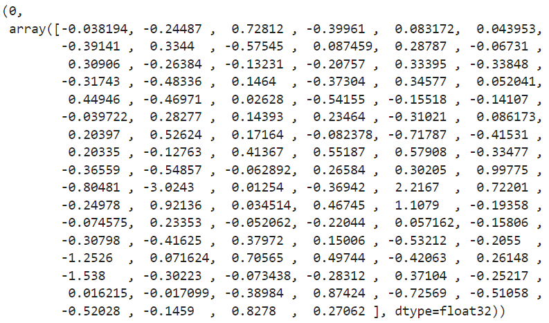

Dataset Preprocessing 

The IMDB dataset obtained through the loader has undergone word segmentation, but it requires additional preprocessing to be suitable for constructing training data. This preprocessing encompasses two main steps: 

• All tokens are converted to index IDs via the Vocab interface.  
• Text sequences are standardized to a uniform length; sequences that are too short are filled with <pad>, while longer sequences are truncated. 

The preprocessing is performed using interfaces provided within the mindspore.dataset module. All these interfaces are part of MindSpore's high-performance data engine, with each interface's operation considered a segment of the data pipeline. Firstly, the text.Lookup interface is used for the table lookup operation that converts tokens to index IDs, loading the previously constructed vocabulary and specifying the unknown_token. Secondly, to unify the length of the text sequence, we use the PadEnd interface, which stipulates a maximum length (in this case, 500) and a padding value. Here, the padding value corresponds to the index ID of the <pad> marker in the vocabulary. textIn addition to preprocessingthe data set , due to the need for subsequent model training,labelthe data must be converted to float32 format. 

import mindspore as ms

lookup_op = ds.text.Lookup(vocab, unknown_token='<unk>')
pad_op = ds.transforms.PadEnd([500], pad_value=vocab.tokens_to_ids('<pad>'))
type_cast_op = ds.transforms.TypeCast(ms.float32)复制

Once the preprocessing operation is concluded, it should be incorporated into the dataset processing pipeline. The `map` interface is used for this purpose, adding operations to the specified column. Since the original IMDB dataset does not contain a validation set, it's divided manually into training and validation sets, at a ratio of 0.7 to 0.3, respectively. Finally, the batch size of the dataset is defined through the `batch` interface, which also includes an option to determine whether or not to discard any residual data that isn't divisible by the set batch size. 

imdb_train = imdb_train.map(operations=[lookup_op, pad_op], input_columns=['text'])
imdb_train = imdb_train.map(operations=[type_cast_op], input_columns=['label'])

imdb_test = imdb_test.map(operations=[lookup_op, pad_op], input_columns=['text'])
imdb_test = imdb_test.map(operations=[type_cast_op], input_columns=['label'])

imdb_train, imdb_valid = imdb_train.split([0.7, 0.3])

imdb_train = imdb_train.batch(64, drop_remainder=True)
imdb_valid = imdb_valid.batch(64, drop_remainder=True)复制

Model Implementation 

I build the convolutional layers utilizing `nn.Conv2d`. The `in_channels` parameter denotes the number of "channels" in your image entering the convolutional layer. In real images, this is typically 3 (one channel each for red, blue, and green), but in text processing, we have only one channel, the text itself. The `out_channels` represents the number of filters, and the `kernel_size` defines the size of the filters. Each of our `kernel_size`s will be [n x emb_dim], where 'n'epresents the size of the n-grams. 

Mindspore expects the input with the batch dimension second for RNNs, whereas for CNNs, it wants the batch dimension first. Fortunately, we don't need to permute the data here since we've already set `batch_first = True` in our `TEXT` field. We then feed the sentence into an embedding layer to obtain our embeddings. The second dimension of the input into a `nn.Conv2d` layer must be the channel dimension. Since text doesn't technically have a channel dimension, we `unsqueeze` our tensor to create one, aligning with our `in_channels=1` in the convolutional layers initialization. 

I subsequently pass the tensors through the convolutional and pooling layers, applying the `ReLU` activation function post-convolution. Another advantage of the pooling layers is their capability to handle sentences of varying lengths. The output size from the convolutional layer depends on its input size, and different batches contain sentences of different lengths. Without the max pooling layer, the input to our linear layer would be dependent on the size of the input sentence, which is not desirable. One way to resolve this would be to trim/pad all sentences to the same length, but with the max pooling layer, we can always expect the input to the linear layer to be the total number of filters. **Note**: there is an exception if your sentences are shorter than the largest filter used. In such cases, you'll have to pad your sentences to match the length of the largest filter. Thankfully, in the IMDb dataset, there are no reviews as short as 5 words, so this isn't a concern for us. But if you're using your own data, you'll need to take this into account. 

Finally, we apply dropout on the concatenated filter outputs, then pass them through a linear layer to make our predictions. 

​

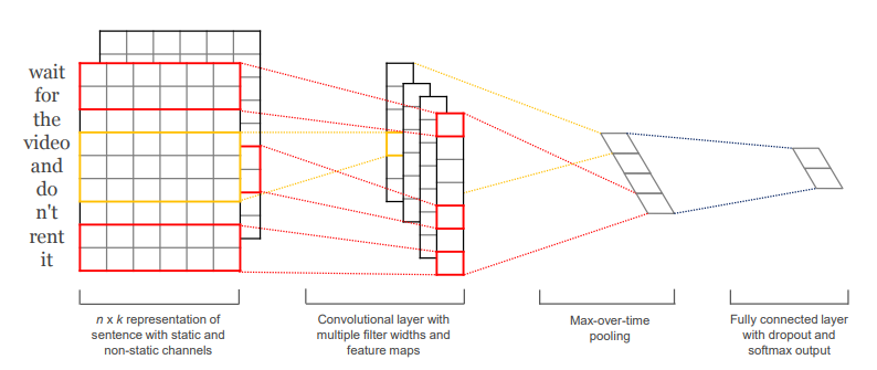
 Figure: Model architecture with two channels for an example sentence. 

from mindspore import Tensor, nn, ops
from mindspore.common.initializer import Normal

class CNN(nn.Cell):
    def __init__(self, embeddings, n_filters, filter_sizes, output_dim, 
                 dropout, pad_idx):
        
        #super(CNN, self).__init__()
        #self.embedding = nn.Embedding(vocab_size, embedding_dim, padding_idx=pad_idx)
        
        super().__init__()
        vocab_size, embedding_dim = embeddings.shape
        self.embedding = nn.Embedding(vocab_size, embedding_dim, embedding_table=ms.Tensor(embeddings), padding_idx=pad_idx)

        self.convs = nn.CellList([
            nn.Conv2d(1, n_filters, (fs, embedding_dim), pad_mode = 'valid', has_bias=True) for fs in filter_sizes
        ])

        self.fc = nn.Dense(len(filter_sizes) * n_filters, output_dim, has_bias=True, weight_init=Normal(0.02))
        
        self.dropout = nn.Dropout(1 - dropout)

        self.relu = nn.ReLU()
        #self.reshape = nn.Reshape()
        self.cat = ops.Concat(axis=1)

    def construct(self, text):
        # embedded = [batch size, 1, sent len, emb dim]
        embedded = self.embedding(text)
        
        embedded = embedded.unsqueeze(1)
        
        squeeze = ops.Squeeze(3)

        conved = [squeeze(self.relu(conv(embedded))) for conv in self.convs]
        squeeze = ops.Squeeze(2)
        #max_pool = nn.MaxPool1d(kernel_size=None)
        pooled = [squeeze(nn.MaxPool1d(kernel_size=conv.shape[2])(conv)) for conv in conved]

        # cat = [batch size, n_filters * len(filter_sizes)]
        cat = self.dropout(self.cat(tuple(pooled)))

        return self.fc(cat)复制

Upon constructing the main structure of the model, we first create an instance of the network based on the designated parameters. Subsequently, we select the loss function and optimizer. Considering the characteristics of the sentiment classification task at hand, which is essentially a binary classification problem aiming to predict 'Positive' or 'Negative', I opt for `nn.BCEWithLogitsLoss`—a binary cross-entropy loss function. 

#INPUT_DIM = len(TEXT.vocab)
#EMBEDDING_DIM = 100
N_FILTERS = 100
FILTER_SIZES = [3,4,5]
OUTPUT_DIM = 1
DROPOUT = 0.5
#PAD_IDX = TEXT.vocab.stoi[TEXT.pad_token]
lr = 0.001
PAD_IDX = vocab.tokens_to_ids('<pad>')

model = CNN(embeddings, N_FILTERS, FILTER_SIZES, OUTPUT_DIM, DROPOUT, PAD_IDX)
loss_fn = nn.BCEWithLogitsLoss(reduction='mean')
optimizer = nn.Adam(model.trainable_params(), learning_rate=lr)
复制

Training Logic 

Once the model is built, we design the training logic. The general training process is broken down into the following steps: 

• Load the data for a Batch; 
• Feed it to the network, perform forward propagation, backpropagation, and update the weights; 
• Return the loss. 

Following this process, we use the `tqdm` library to design a function that trains an epoch, allowing for visualization of the training progress and the associated loss. 

def forward_fn(data, label):
    logits = model(data)
    loss = loss_fn(logits, label)
    return loss

grad_fn = ms.value_and_grad(forward_fn, None, optimizer.parameters)

def train_step(data, label):
    loss, grads = grad_fn(data, label)
    optimizer(grads)
    return loss

def train_one_epoch(model, train_dataset, epoch=0):
    model.set_train()
    total = train_dataset.get_dataset_size()
    loss_total = 0
    step_total = 0
    with tqdm(total=total) as t:
        t.set_description('Epoch %i' % epoch)
        for i in train_dataset.create_tuple_iterator():
            loss = train_step(*i)
            loss_total += loss.asnumpy()
            step_total += 1
            t.set_postfix(loss=loss_total/step_total)
            t.update(1)复制

Evaluation Metrics 

After completing the training logic, we need to evaluate the model. This involves comparing the model's prediction results with the correct labels of the test set to determine prediction accuracy. Given that the sentiment classification of IMDB constitutes a binary classification problem, the classification label (0 or 1) can be obtained by simply rounding off the predicted value. Subsequently, it is enough to check whether it matches the correct label. The following describes the implementation of the accuracy calculation function for binary classification: 

def binary_accuracy(preds, y):
    """
    Calculate the accuracy of each batch.
    """
    # Round off the predicted value.
    rounded_preds = np.around(ops.sigmoid(preds).asnumpy())
    correct = (rounded_preds == y).astype(np.float32)
    acc = correct.sum() / len(correct)
    return acc复制

With the accuracy calculation function in place, we design the evaluation logic, which is similar to the training logic. The steps are as follows: 

• Load the data for a Batch; 
• Feed it to the network, perform forward propagation, and obtain the predicted result; 
• Calculate the accuracy. 

def evaluate(model, test_dataset, criterion, epoch=0):
    total = test_dataset.get_dataset_size()
    epoch_loss = 0
    epoch_acc = 0
    step_total = 0
    model.set_train(False)

    with tqdm(total=total) as t:
        t.set_description('Epoch %i' % epoch)
        for i in test_dataset.create_tuple_iterator():
            predictions = model(i[0])
            loss = criterion(predictions, i[1])
            epoch_loss += loss.asnumpy()

            acc = binary_accuracy(predictions, i[1])
            epoch_acc += acc

            step_total += 1
            t.set_postfix(loss=epoch_loss/step_total, acc=epoch_acc/step_total)
            t.update(1)

    return epoch_loss / total
复制

Model Training 

Having completed the model buliding, as well as the design of the training and evaluation logic, we proceed to the model training. Here, we set the number of training epochs to 5. Concurrently, we maintain a variable `best_valid_loss` to store the optimal model. Based on the loss value of each epoch during evaluation, the epoch with the smallest loss value is chosen to save the model. 

num_epochs = 5
best_valid_loss = float('inf')
ckpt_file_name = os.path.join(cache_dir, 'analysis.ckpt')

for epoch in range(num_epochs):
    train_one_epoch(model, imdb_train, epoch)
    valid_loss = evaluate(model, imdb_valid, loss_fn, epoch)

    if valid_loss < best_valid_loss:
        best_valid_loss = valid_loss
        ms.save_checkpoint(model, ckpt_file_name)复制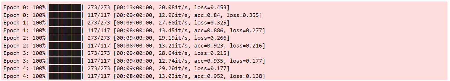

Model Testing 

Once the training of the model is concluded, it is typically required to either test the model or deploy it online. During this phase, it is necessary to load the saved optimal model (checkpoint) for any forthcoming testing. We accomplish this by leveraging the Checkpoint loading and network weight loading interfaces supplied by MindSpore: 

• Retrieve the saved model Checkpoint into memory, 
• Incorporate the Checkpoint into the model. 

param_dict = ms.load_checkpoint(ckpt_file_name)
ms.load_param_into_net(model, param_dict)

imdb_test = imdb_test.batch(64)
evaluate(model, imdb_test, loss_fn)
复制

That's excellent! Achieving an accuracy rate comparable to that stated in the original paper is a strong validation of the model's performance.  

Custom Input Test 

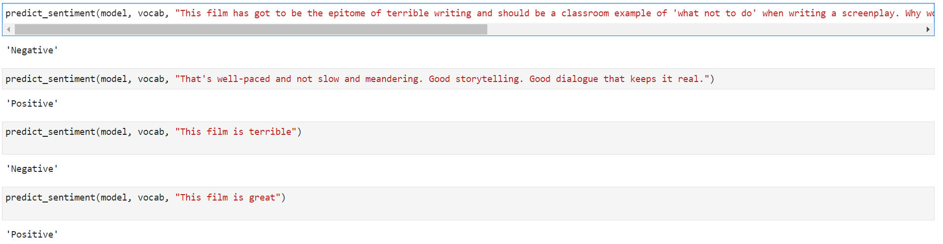
 Lastly, we design a prediction function to achieve the initially described functionality: input a review sentence and obtain the sentiment classification for that review. The steps specifically include: 

1. Pad Sentence: The function `pad_sentence` takes a sentence, converts it to lowercase and splits it into tokens. If the length of the tokenized sentence is less than the maximum length, it appends padding tokens (`<pad>`) to the sentence until it reaches the maximum length. If the sentence is longer than the maximum length, it is truncated. 

2. Map Scores to Sentiments: `score_map` is a dictionary mapping scores (1 or 0) to their corresponding sentiments ("Positive" or "Negative"). 

3. Predict Sentiment: The function `predict_sentiment` is designed to predict the sentiment of a given sentence. It follows the steps: 

• Set the model to evaluation mode with `model.set_train(False)`. 
• Pad the input sentence using the `pad_sentence` function. 
• Convert the tokenized sentence to its corresponding indexes using the vocabulary. 
• Convert the indexed sentence into a tensor and add a new dimension to match the input shape of the model. 
• Pass the tensor to the model and obtain the prediction. 
• Convert the prediction into a sentiment by applying a sigmoid function, rounding the result, converting it to an integer, and looking up the corresponding sentiment in the `score_map`. 

4. Return Sentiment: The function finally returns the sentiment of the given sentence as predicted by the model. 

def pad_sentence(sentence, max_length, pad_token='<pad>'):
    tokenized = sentence.lower().split()
    
    if len(tokenized) < max_length:
        tokenized += [pad_token] * (max_length - len(tokenized))
    else:
        tokenized = tokenized[:max_length]
    
    return tokenized

score_map = {
    1: "Positive",
    0: "Negative"
}

def predict_sentiment(model, vocab, sentence, max_length=500):
    model.set_train(False)
    
    # Pad sentence
    tokenized = pad_sentence(sentence, max_length)
    
    # Convert tokens to ids
    indexed = [vocab.tokens_to_ids(token) for token in tokenized]
    
    # Create tensor and expand dims
    tensor = ms.Tensor(indexed, ms.int32)
    tensor = tensor.expand_dims(0)
    
    # Predict sentiment
    prediction = model(tensor)
    
    # Convert prediction to sentiment
    sentiment = score_map[int(np.round(ops.sigmoid(prediction).asnumpy()))]
    
    return sentiment
复制

 

 Thank you. 

ንጉስ ዳዊት በቃሉ

The full code is available in Jupyter Notebook and Python file format on my Gitee here.