YOLOV2翻译

YOLO9000: Better, Faster, Stronger

Joseph Redmon×, Ali Farhadi†×

University of Washington, Allen Institute for AI†, XNOR.ai×

http://pjreddie.com/yolo9000/

Abstract

We introduce YOLO9000, a state-of-the-art, real-time object detection system that can detect over 9000 object categories. First we propose various improvements to the YOLO detection method, both novel and drawn from prior work. The improved model, YOLOv2, is state-of-the-art on standard detection tasks like PASCAL VOC and COCO. Using a novel, multi scale training method the same YOLOv2 model can run at varying sizes, offering an easy tradeoff between speed and accuracy. At 67 FPS, YOLOv2 gets 76.8 mAP on VOC 2007. At 40 FPS, YOLOv2 gets 78.6 mAP, outperforming state-of-the-art methods like Faster R-CNN with ResNet and SSD while still running significantly faster. Finally we propose a method to jointly train on object detection and classification. Using this method we train YOLO9000 simultaneously on the COCO detection dataset and the ImageNet classification dataset. Our joint training allows YOLO9000 to predict detections for object classes that don’t have labelled detection data. We validate our approach on the ImageNet detection task. YOLO9000 gets 19.7 mAP on the ImageNet detection validation set despite only having detection data for 44 of the 200 classes. On the 156 classes not in COCO, YOLO9000 gets 16.0 mAP. YOLO9000 predicts detections for more than 9000 different object categories, all in real-time.

我们介绍的 YOLO9000 是最先进的实时目标检测系统，可检测 9000 多个目标类别。首先，我们对 YOLO 检测方法提出了各种改进建议，其中既有新颖之处，也有借鉴先前研究成果的地方。改进后的模型 YOLOv2 在标准检测任务（如 PASCAL VOC 和 COCO）中处于一流水平。利用新颖的多尺度训练方法，同一 YOLOv2 模型可以在不同的尺寸下运行，从而在速度和准确性之间轻松做出权衡。在 67 FPS 下，YOLOv2 在 VOC 2007 上获得了 76.8 mAP。在 40 FPS 时，YOLOv2 可获得 78.6 mAP，超过了最先进的方法，如使用 ResNet 和 SSD 的 Faster R-CNN，同时运行速度也明显更快。最后，我们提出了一种联合训练目标检测和分类的方法。利用这种方法，我们在 COCO 检测数据集和 ImageNet 分类数据集上同时训练 YOLO9000。通过联合训练，YOLO9000 可以预测没有标注检测数据的目标类别的检测结果。我们在 ImageNet 检测任务中验证了我们的方法。尽管只有 200 个类别中 44 个类别的检测数据，但 YOLO9000 在 ImageNet 检测验证集上获得了 19.7 mAP。在 COCO 以外的 156 个类别中，YOLO9000 获得了 16.0 mAP。YOLO9000 可实时预测 9000 多个不同目标类别的检测结果。

1 Introduction

General purpose object detection should be fast, accurate, and able to recognize a wide variety of objects. Since the introduction of neural networks, detection frameworks have become increasingly fast and accurate. However, most detection methods are still constrained to a small set of objects.

通用目标检测应该快速、准确，并能识别各种各样的目标。自从引入神经网络以来，检测框架变得越来越快速和准确。然而，大多数检测方法仍局限于一小部分目标。

Current object detection datasets are limited compared to datasets for other tasks like classification and tagging. The most common detection datasets contain thousands to hundreds of thousands of images with dozens to hundreds of tags [3] [10] [2]. Classification datasets have millions of images with tens or hundreds of thousands of categories[20] [2].

与分类和标记等其他任务的数据集相比，当前的目标检测数据集十分有限。最常见的检测数据集包含数千到数十万张图像，以及数十到数百个标签 [3] [10] [2]。分类数据集则包含数百万张图片和数万或数十万个类别[20] [2]。

We would like detection to scale to level of object classification. However, labelling images for detection is far more expensive than labelling for classification or tagging (tags are often user-supplied for free). Thus we are unlikely to see detection datasets on the same scale as classification datasets in the near future.

我们希望检测能达到目标分类的水平。然而，为检测而标记图像的成本远高于为分类或标记而标记图像的成本（标记通常由用户免费提供）。因此，在不久的将来，我们不太可能看到与分类数据集同等规模的检测数据集。

We propose a new method to harness the large amount of classification data we already have and use it to expand the scope of current detection systems. Our method uses a hierarchical view of object classification that allows us to combine distinct datasets together.

我们提出了一种新方法来利用我们已有的大量分类数据，并用它来扩展当前检测系统的范围。我们的方法采用了物体分类的分层视图，允许我们将不同的数据集结合在一起。

We also propose a joint training algorithm that allows us to train object detectors on both detection and classification data. Our method leverages labeled detection images to learn to precisely localize objects while it uses classification images to increase its vocabulary and robustness.

我们还提出了一种联合训练算法，允许我们在检测和分类数据上训练目标检测器。我们的方法利用标记检测图像来学习精确定位目标，同时利用分类图像来增加其词汇量和鲁棒性。

Using this method we train YOLO9000, a real-time object detector that can detect over 9000 different object categories. First we improve upon the base YOLO detection system to produce YOLOv2, a state-of-the-art, real-time detector. Then we use our dataset combination method and joint training algorithm to train a model on more than 9000 classes from ImageNet as well as detection data from COCO. All of our code and pre-trained models are available online at http://pjreddie.com/yolo9000/.

利用这种方法，我们训练了 YOLO9000，这是一种实时目标检测器，可以检测出 9000 多种不同的目标类别。首先，我们改进了基础 YOLO 检测系统，生成了 YOLOv2，这是一款最先进的实时检测器。然后，我们使用数据集组合方法和联合训练算法，对 ImageNet 的 9000 多个类别以及 COCO 的检测数据进行模型训练。我们的所有代码和预训练模型都可在 http://pjreddie.com/yolo9000/ 上在线获取。

2 Better

YOLO suffers from a variety of shortcomings relative to state-of-the-art detection systems. Error analysis of YOLO compared to Fast R-CNN shows that YOLO makes a significant number of localization errors. Furthermore, YOLO has relatively low recall compared to region proposal-based methods. Thus we focus mainly on improving recall and localization while maintaining classification accuracy.

与最先进的检测系统相比，YOLO 存在多种缺陷。对 YOLO 与快速 R-CNN 的误差分析表明，YOLO 存在大量定位误差。此外，与基于region proposal 的方法相比，YOLO 的召回率相对较低。因此，我们主要关注在保持分类准确性的同时提高召回率和定位率。

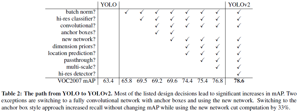
Computer vision generally trends towards larger, deeper networks [6] [18] [17]. Better performance often hinges on training larger networks or ensembling multiple models together. However, with YOLOv2 we want a more accurate detector that is still fast. Instead of scaling up our network, we simplify the network and then make the representation easier to learn. We pool a variety of ideas from past work with our own novel concepts to improve YOLO’s performance. A summary of results can be found in Table 2.

计算机视觉通常倾向于使用更大、更深的网络 [6] [18] [17]。更好的性能往往取决于训练更大的网络或将多个模型组合在一起。然而，对于 YOLOv2，我们希望能有一个更精确的检测器，同时速度仍然很快。与其扩大网络规模，我们不如简化网络，然后让表示更易于学习。我们将过去工作中的各种想法与我们自己的新概念结合起来，以提高 YOLO 的性能。结果汇总见表 2。

Batch Normalization. Batch normalization leads to significant improvements in convergence while eliminating the need for other forms of regularization [7]. By adding batch normalization on all of the convolutional layers in YOLO we get more than 2% improvement in mAP. Batch normalization also helps regularize the model. With batch normalization we can remove dropout from the model without overfitting.

Batch Normalization。批量归一化可显著提高收敛性，同时无需其他形式的正则化[7]。通过在 YOLO 的所有卷积层上添加批量归一化，我们的 mAP 提高了 2% 以上。批量归一化还有助于对模型进行正则化。通过批量归一化，我们可以在不过度拟合的情况下消除模型中的遗漏。

High Resolution Classifier. All state-of-the-art detection methods use classifier pre-trained on ImageNet [16]. Starting with AlexNet most classifiers operate on input images smaller than 256 × 256 [8]. The original YOLO trains the classifier network at 224 × 224 and increases the resolution to 448 for detection. This means the network has to simultaneously switch to learning object detection and adjust to the new input resolution.

High Resolution Classifier. 所有先进的检测方法都使用在 ImageNet 上预先训练好的分类器 [16]。从 AlexNet 开始，大多数分类器都能在小于 256 × 256 的输入图像上运行 [8]。最初的 YOLO 以 224 × 224 的分辨率训练分类器网络，并将检测分辨率提高到 448。这意味着网络必须同时切换到学习目标检测，并适应新的输入分辨率。

For YOLOv2 we first fine tune the classification network at the full 448×448 resolution for 10 epochs on ImageNet. This gives the network time to adjust its filters to work better on higher resolution input. We then fine tune the resulting network on detection. This high resolution classification network gives us an increase of almost 4% mAP.

对于 YOLOv2，我们首先在 ImageNet 上以完整的 448×448 分辨率对分类网络进行 10 次微调。这让网络有时间调整其过滤器，以便在更高分辨率的输入上更好地工作。然后，我们在检测时对由此产生的网络进行微调。这种高分辨率分类网络使我们的 mAP 提高了近 4%。

Convolutional With Anchor Boxes. YOLO predicts the coordinates of bounding boxes directly using fully connected layers on top of the convolutional feature extractor.

带锚框的卷积网络。YOLO 在卷积特征提取器的基础上使用全连接层直接预测框的坐标。

Instead of predicting coordinates directly Faster R-CNN predicts bounding boxes using hand-picked priors [15]. Using only convolutional layers the region proposal network (RPN) in Faster R-CNN predicts offsets and confidences for anchor boxes. Since the prediction layer is convolutional, the RPN predicts these offsets at every location in a feature map. Predicting offsets instead of coordinates simplifies the problem and makes it easier for the network to learn.

Faster R-CNN 不直接预测坐标，而是使用手工挑选的前验[15]来预测边界框。Faster R-CNN 中的区域建议网络（RPN）仅使用卷积层来预测锚点框的偏移和置信度。由于预测层是卷积层，因此 RPN 可以预测特征图中每个位置的偏移量。预测偏移量而不是坐标简化了问题，使网络更容易学习。

We remove the fully connected layers from YOLO and use anchor boxes to predict bounding boxes. First we eliminate one pooling layer to make the output of the network’s convolutional layers higher resolution. We also shrink the network to operate on 416 input images instead of 448×448. We do this because we want an odd number of locations in our feature map so there is a single center cell. Objects, especially large objects, tend to occupy the center of the image so it’s good to have a single location right at the center to predict these objects instead of four locations that are all nearby. YOLO’s convolutional layers downsample the image by a factor of 32 so by using an input image of 416 we get an output feature map of 13 × 13.

我们从 YOLO 中移除全连接层，使用锚框来预测边界框。首先，我们取消了一个汇集层，使网络卷积层的输出分辨率更高。我们还缩小了网络，使其能在 416 幅而非 448×448 幅输入图像上运行。之所以这样做，是因为我们希望特征图中的位置数量为奇数，这样就有了一个中心单元。物体，尤其是大型物体，往往会占据图像的中心位置，因此最好在中心位置设置一个位置来预测这些物体，而不是在附近设置四个位置。YOLO 的卷积层会对图像进行 32 倍的下采样，因此使用 416 的输入图像，我们可以得到 13 × 13 的输出特征图。

When we move to anchor boxes we also decouple the class prediction mechanism from the spatial location and instead predict class and objectness for every anchor box. Following YOLO, the objectness prediction still predicts the IOU of the ground truth and the proposed box and the class predictions predict the conditional probability of that class given that there is an object.

当我们移动到锚点框时，我们也将类别预测机制与空间位置解耦，转而预测每个锚点框的类别和对象性。按照 YOLO 的方法，对象性预测仍然是预测 ground truth 和提议框的 IOU，而类别预测则是预测在有对象的情况下该类别的条件概率。

Using anchor boxes we get a small decrease in accuracy. YOLO only predicts 98 boxes per image but with anchor boxes our model predicts more than a thousand. Without anchor boxes our intermediate model gets 69.5 mAP with a recall of 81%. With anchor boxes our model gets 69.2 mAP with a recall of 88%. Even though the mAP decreases, the increase in recall means that our model has more room to improve.

使用锚文本框后，准确率略有下降。YOLO 只预测了每幅图像中的 98 个预测框，但使用锚点框后，我们的模型预测出了一千多个预测框。在不使用锚点框的情况下，我们的中间模型获得了 69.5 mAP，召回率为 81%。使用锚点框后，我们的模型获得了 69.2 mAP，召回率为 88%。尽管 mAP 有所下降，但召回率的提高意味着我们的模型还有更大的改进空间。

Dimension Clusters. We encounter two issues with anchor boxes when using them with YOLO. The first is that the box dimensions are hand picked. The network can learn to adjust the boxes appropriately but if we pick better priors for the network to start with we can make it easier for the network to learn to predict good detections.

维度集群。在将锚点框与 YOLO 一起使用时，我们遇到了两个问题。首先，锚点框的维度是人工挑选的。网络可以通过学习来适当调整锚点框，但如果我们一开始就为网络挑选更好的前验，就能让网络更容易学会预测好的检测结果。

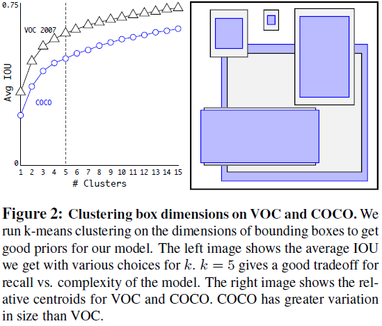
Instead of choosing priors by hand, we run k-means clustering on the training set bounding boxes to automatically find good priors. If we use standard k-means with Euclidean distance larger boxes generate more error than smaller boxes. However, what we really want are priors that lead to good IOU scores, which is independent of the size of the box. Thus for our distance metric we use:

我们不用手工选择先验值，而是在训练集的边界框上运行 k-means 聚类，自动找到好的先验值。如果我们使用标准的欧氏距离 k-means，较大的方框会比较小的方框产生更多误差。然而，我们真正需要的是能带来良好 IOU 分数的先验值，这与方框的大小无关。因此，我们使用以下距离度量:
$$d(box,centroid)=1-IOU(box,centroid)$$
We run k-means for various values of k and plot the average IOU with closest centroid, see Figure 2. We choose k = 5 as a good tradeoff between model complexity and high recall. The cluster centroids are significantly different than hand-picked anchor boxes. There are fewer short, wide boxes and more tall, thin boxes.

我们在不同的 k 值下运行 k-means，并绘制出最接近中心点的平均 IOU，见图 2。我们选择 k = 5 作为模型复杂性和高召回率之间的良好权衡。聚类中心点与手工挑选的锚框有明显不同。短而宽的方框较少，高而细的方框较多。

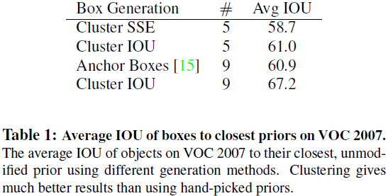
We compare the average IOU to closest prior of our clustering strategy and the hand-picked anchor boxes in Table 1. At only 5 priors the centroids perform similarly to 9 anchor boxes with an average IOU of 61.0 compared to 60.9. If we use 9 centroids we see a much higher average IOU. This indicates that using k-means to generate our bounding box starts the model off with a better representation and makes the task easier to learn.

我们在表 1 中比较了我们的聚类策略和手工挑选的锚点的平均 IOU 与最接近先验的比较。在只有 5 个先验时，中心点的表现与 9 个锚点相似，平均 IOU 为 61.0，而 9 个锚点为 60.9。如果使用 9 个中心点，平均 IOU 则要高得多。这表明，使用 k-means 生成边界框可以让模型以更好的表现形式启动，并使任务更容易学习。

Direct location prediction. When using anchor boxes with YOLO we encounter a second issue: model instability, especially during early iterations. Most of the instability comes from predicting the (x, y) locations for the box. In region proposal networks the network predicts values $t_x$ and $t_y$ and the (x, y) center coordinates are calculated as:

直接位置预测。在使用锚点盒和 YOLO 时，我们会遇到第二个问题：模型不稳定，尤其是在早期迭代时。大部分不稳定性来自于预测框的 (x, y) 位置。在区域建议网络中，网络预测值为 $t_x$ 和 $t_y$，（x, y）中心坐标的计算公式为
$$\begin{gathered} x=(t_x\ast w_a)-x_a \\ y=(t_y\ast h_a)-y_a \end{gathered}$$
For example, a prediction of $t_x=1$ would shift the box to the right by the width of the anchor box, a prediction of $t_x=-1$ would shift it to the left by the same amount.

例如，预测 $t_x=1$ 时，框会向右移动锚点框的宽度，预测 $t_x=-1$ 时，框会向左移动相同的宽度。

This formulation is unconstrained so any anchor box can end up at any point in the image, regardless of what location predicted the box. With random initialization the model takes a long time to stabilize to predicting sensible offsets.

这个公式是无约束的，因此任何锚点框都可以在图像中的任何一点结束，而不管是哪个位置预测了这个框。在随机初始化的情况下，模型需要很长时间才能稳定到预测合理的偏移量。

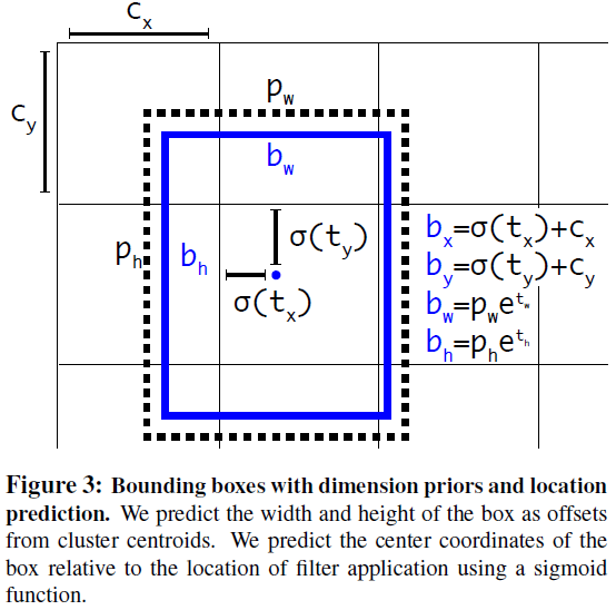
Instead of predicting offsets we follow the approach of YOLO and predict location coordinates relative to the location of the grid cell. This bounds the ground truth to fall between 0 and 1. We use a logistic activation to constrain the network’s predictions to fall in this range.

我们采用 YOLO 方法，预测相对于网格单元位置的位置坐标，而不是预测偏移量。这就将 ground truth 限定在 0 和 1 之间。我们使用逻辑激活来限制网络的预测值在此范围内。

The network predicts 5 bounding boxes at each cell in the output feature map. The network predicts 5 coordinates for each bounding box,$ t_x, t_y, t_w, t_h$, and to. If the cell is offset from the top left corner of the image by (cx, cy) and the bounding box prior has width and height pw, ph, then the predictions correspond to:

网络会在输出特征图中的每个单元预测 5 个边界框。网络会为每个预测框预测 5 个坐标：$ t_x、t_y、t_w、t_h$ 和 to。如果单元格与图像左上角的偏移量为 (cx，cy)，且边界框的先验值为宽和高 pw，ph，则预测结果对应于：
$$\begin{gathered} b_x=\sigma (t_x)+c_x \\ {b}_x=\sigma (t_y)+c_y \\ {b}_w=p_w{e}^{t_w} \\ {b}_h=p_h{e}^{t_h} \\ Pr(object)\ast IOU(b,pbject)=\sigma (t_o) \end{gathered}$$
Since we constrain the location prediction the parametrization is easier to learn, making the network more stable. Using dimension clusters along with directly predicting the bounding box center location improves YOLO by almost 5% over the version with anchor boxes.

由于我们对位置预测进行了限制，因此参数化更容易学习，从而使网络更加稳定。使用维度集群并直接预测边界框中心位置，可使 YOLO 比使用锚点框的版本提高近 5%。

Fine-Grained Features. This modified YOLO predicts detections on a 13 × 13 feature map. While this is sufficient for large objects, it may benefit from finer grained features for localizing smaller objects. Faster R-CNN and SSD both run their proposal networks at various feature maps in the network to get a range of resolutions. We take a different approach, simply adding a passthrough layer that brings features from an earlier layer at 26 × 26 resolution.

细粒度特征。改进后的 YOLO 可预测 13 × 13 特征图上的检测结果。虽然这对于大型物体来说已经足够，但在定位较小物体时，它可能会受益于更精细的特征。Faster R-CNN 和 SSD 都在网络中的不同特征图上运行其建议网络，以获得一系列分辨率。我们采用了一种不同的方法，即简单地添加一个直通层，将先前层中的特征以 26 × 26 的分辨率进行处理。

The passthrough layer concatenates the higher resolution features with the low resolution features by stacking adjacent features into different channels instead of spatial locations, similar to the identity mappings in ResNet. This turns the 26 × 26 × 512 feature map into a 13 × 13 × 2048 feature map, which can be concatenated with the original features. Our detector runs on top of this expanded feature map so that it has access to fine grained features. This gives a modest 1% performance increase.

直通层通过将相邻特征堆叠到不同通道而非空间位置，将高分辨率特征与低分辨率特征连接起来，类似于 ResNet 中的身份映射。这样，26 × 26 × 512 的特征图就变成了 13 × 13 × 2048 的特征图，可以与原始特征图连接起来。我们的检测器运行在这个扩展的特征图之上，因此可以访问细粒度特征。这样，性能略微提高了 1%。

Multi-Scale Training. The original YOLO uses an input resolution of 448 × 448. With the addition of anchor boxes we changed the resolution to 416×416. However, since our model only uses convolutional and pooling layers it can be resized on the fly. We want YOLOv2 to be robust to running on images of different sizes so we train this into the model.

多尺度训练。最初的 YOLO 使用 448 × 448 的输入分辨率。增加锚点框后，我们将分辨率改为 416×416。不过，由于我们的模型只使用卷积层和池化层，因此可以即时调整大小。我们希望 YOLOv2 能够在不同尺寸的图像上稳健运行，因此我们在模型中训练了这一点。

Instead of fixing the input image size we change the network every few iterations. Every 10 batches our network randomly chooses new image dimensions. Since our model downsamples by a factor of 32, we pull from the following multiples of 32: {320, 352, …, 608}. Thus the smallest option is 320×320 and the largest is 608×608. We resize the network to that dimension and continue training.

我们没有固定输入图像的大小，而是每迭代几次就改变网络一次。每 10 次迭代，我们的网络会随机选择新的图像尺寸。由于我们的模型是按 32 倍进行降采样的，因此我们从以下 32 的倍数中选择：{320, 352, …, 608}。因此，最小的选项是 320×320，最大的是 608×608。我们将网络的大小调整到该维度，然后继续训练。

This regime forces the network to learn to predict well across a variety of input dimensions. This means the same network can predict detections at different resolutions. The network runs faster at smaller sizes so YOLOv2 offers an easy tradeoff between speed and accuracy.

这种机制迫使网络学会在各种输入维度上进行良好的预测。这意味着同一个网络可以预测不同分辨率下的检测结果。网络在较小的尺寸下运行速度更快，因此 YOLOv2 可以在速度和准确性之间轻松做出权衡。

At low resolutions YOLOv2 operates as a cheap, fairly accurate detector. At 288×288 it runs at more than 90 FPS with mAP almost as good as Fast R-CNN. This makes it ideal for smaller GPUs, high framerate video, or multiple video streams.

在低分辨率下，YOLOv2 是一种廉价、相当精确的检测器。在 288×288 分辨率下，它的运行速度超过 90 FPS，mAP 几乎与快速 R-CNN 不相上下。这使它成为较小 GPU、高帧率视频或多视频流的理想选择。

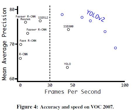
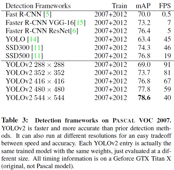
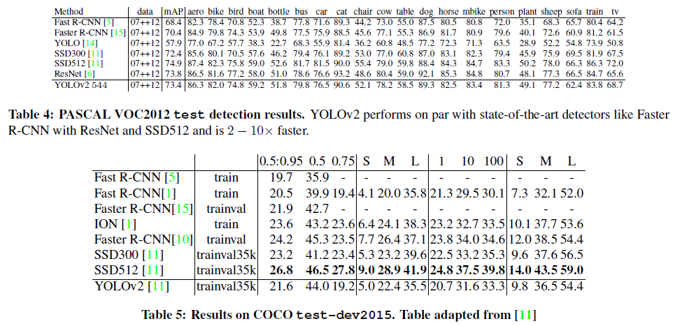
At high resolution YOLOv2 is a state-of-the-art detector with 78.6 mAP on VOC 2007 while still operating above real-time speeds. See Table 3 for a comparison of YOLOv2 with other frameworks on VOC 2007. Figure 4 Further Experiments. We train YOLOv2 for detection on VOC 2012. Table 4 shows the comparative performance of YOLOv2 versus other state-of-the-art detection systems. YOLOv2 achieves 73.4 mAP while running far faster than other methods. We also train on COCO, see Table 5. On the VOC metric (IOU = .5) YOLOv2 gets 44.0 mAP, comparable to SSD and Faster R-CNN.

在高分辨率下，YOLOv2 是最先进的检测器，在 VOC 2007 上的 mAP 为 78.6，同时运行速度仍高于实时速度。有关 YOLOv2 与 VOC 2007 上其他框架的比较，请参见表 3。图 4 进一步实验。我们在 VOC 2012 上训练 YOLOv2 进行检测。表 4 显示了 YOLOv2 与其他一流检测系统的性能比较。YOLOv2 实现了 73.4 mAP，运行速度远远超过其他方法。我们还对 COCO 进行了训练，见表 5。在 VOC 指标（IOU = .5）上，YOLOv2 获得了 44.0 mAP，与 SSD 和 Faster R-CNN 不相上下。

3 Faster

We want detection to be accurate but we also want it to be fast. Most applications for detection, like robotics or self driving cars, rely on low latency predictions. In order to maximize performance we design YOLOv2 to be fast from the ground up.

我们希望检测准确，但也希望检测快速。大多数检测应用（如机器人或自动驾驶汽车）都依赖于低延迟预测。为了最大限度地提高性能，我们设计的 YOLOv2 从一开始就非常快。

Most detection frameworks rely on VGG-16 as the base feature extractor [17]. VGG-16 is a powerful, accurate classification network but it is needlessly complex. The convolutional layers of VGG-16 require 30.69 billion floating point operations for a single pass over a single image at 224 × 224 resolution.

大多数检测框架都依赖 VGG-16 作为基础特征提取器[17]。VGG-16 是一个功能强大、准确的分类网络，但它的复杂性却毋庸置疑。VGG-16 的卷积层需要 306.9 亿次浮点运算，才能在 224 × 224 分辨率下对单幅图像进行一次处理。

The YOLO framework uses a custom network based on the Googlenet architecture [19]. This network is faster than VGG-16, only using 8.52 billion operations for a forward pass. However, it’s accuracy is slightly worse than VGG-16 For single-crop, top-5 accuracy at 224 × 224, YOLO’s custom model gets 88.0% ImageNet compared to 90.0% for VGG-16.

YOLO 框架使用的是基于 Googlenet 架构的定制网络[19]。该网络的速度比 VGG-16 更快，一次前向扫描仅需 85.2 亿次运算。不过，它的准确率略低于 VGG-16。在 224 × 224 分辨率下，YOLO 的自定义模型获得了 88.0% 的 ImageNet 准确率，而 VGG-16 为 90.0%。

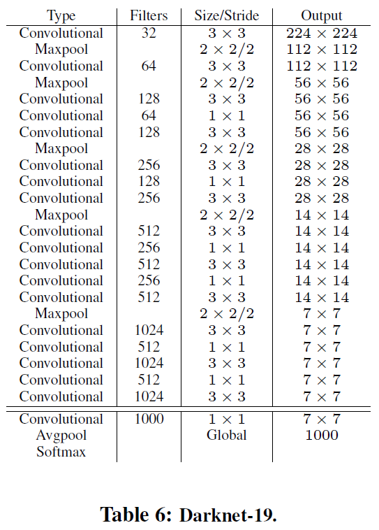
Darknet-19. We propose a new classification model to be used as the base of YOLOv2. Our model builds off of prior work on network design as well as common knowledge in the field. Similar to the VGG models we use mostly 3 × 3 filters and double the number of channels after every pooling step [17]. Following the work on Network in Network (NIN) we use global average pooling to make predictions as well as 1 × 1 filters to compress the feature representation between 3 × 3 convolutions [9]. We use batch normalization to stabilize training, speed up convergence,and regularize the model [7].

Darknet-19。我们提出了一个新的分类模型，作为 YOLOv2 的基础。我们的模型建立在先前的网络设计工作以及该领域的常识基础之上。与 VGG 模型类似，我们主要使用 3 × 3 过滤器，并在每个池化步骤后将通道数量增加一倍[17]。根据网络中的网络（NIN）的研究成果，我们使用全局平均池进行预测，并使用 1 × 1 过滤器来压缩 3 × 3 卷积之间的特征表示[9]。我们使用批量归一化来稳定训练，加快收敛速度，并对模型进行正则化处理 [7]。

Our final model, called Darknet-19, has 19 convolutional layers and 5 maxpooling layers. For a full description see Table 6. Darknet-19 only requires 5.58 billion operations to process an image yet achieves 72.9% top-1 accuracy and 91.2% top-5 accuracy on ImageNet.

我们的最终模型名为 Darknet-19，有 19 个卷积层和 5 个 maxpooling 层。完整描述见表 6。Darknet-19 处理一幅图像只需要 55.8 亿次运算，但在 ImageNet 上却达到了 72.9% 的前 1 级准确率和 91.2% 的前 5 级准确率。

Training for classification. We train the network on the standard ImageNet 1000 class classification dataset for 160 epochs using stochastic gradient descent with a starting learning rate of 0.1, polynomial rate decay with a power of 4, weight decay of 0.0005 and momentum of 0.9 using the Darknet neural network framework [13]. During training we use standard data augmentation tricks including random crops, rotations, and hue, saturation, and exposure shifts.

分类训练 我们使用 Darknet 神经网络框架[13]，以 0.1 的起始学习率、4 次幂的多项式速率衰减、0.0005 的权重衰减和 0.9 的动量，在标准 ImageNet 1000 类分类数据集上对网络进行了 160 个历元的训练。在训练过程中，我们使用了标准的数据增强技巧，包括随机裁剪、旋转以及色调、饱和度和曝光度的变化。

As discussed above, after our initial training on images at 224 × 224 we fine tune our network at a larger size, 448. For this fine tuning we train with the above parameters but for only 10 epochs and starting at a learning rate of 10−3. At this higher resolution our network achieves a top-1 accuracy of 76.5% and a top-5 accuracy of 93.3%.

如上所述，在 224 × 224 尺寸的图像上进行初始训练后，我们将在更大的 448 尺寸上对网络进行微调。在微调时，我们使用上述参数进行训练，但只训练 10 次，学习率为 10-3。在这一更高分辨率下，我们的网络达到了 76.5% 的前 1 级准确率和 93.3% 的前 5 级准确率。

Training for detection. We modify this network for detection by removing the last convolutional layer and instead adding on three 3 × 3 convolutional layers with 1024 filters each followed by a final 1 × 1 convolutional layer with the number of outputs we need for detection. For VOC we predict 5 boxes with 5 coordinates each and 20 classes per box so 125 filters. We also add a passthrough layer from the final 3 × 3 × 512 layer to the second to last convolutional layer so that our model can use fine grain features.

检测训练。我们去掉了最后一个卷积层，增加了三个 3 × 3 卷积层，每个卷积层有 1024 个滤波器，然后再增加一个 1 × 1 卷积层，最后一个卷积层的输出数与检测所需的输出数相同。对于 VOC，我们预测 5 个框，每个框有 5 个坐标，每个框有 20 个类别，因此有 125 个滤波器。我们还从最后的 3 × 3 × 512 层添加了一个直通层到倒数第二个卷积层，这样我们的模型就可以使用细粒度特征。

We train the network for 160 epochs with a starting learning rate of 10−3, dividing it by 10 at 60 and 90 epochs. We use a weight decay of 0.0005 and momentum of 0.9. We use a similar data augmentation to YOLO and SSD with random crops, color shifting, etc. We use the same training strategy on COCO and VOC.

我们以 10-3 的起始学习率对网络进行了 160 个历元的训练，并在 60 和 90 个历元时将学习率除以 10。我们使用的权重衰减为 0.0005，动量为 0.9。我们使用了与 YOLO 和 SSD 类似的数据增强方法，包括随机裁剪、颜色偏移等。我们对 COCO 和 VOC 采用相同的训练策略。

4 Stronger

We propose a mechanism for jointly training on classification and detection data. Our method uses images labelled for detection to learn detection-specific information like bounding box coordinate prediction and objectness as well as how to classify common objects. It uses images with only class labels to expand the number of categories it can detect.

我们提出了一种对分类和检测数据进行联合训练的机制。我们的方法使用贴有检测标签的图像来学习特定的检测信息，如预测框坐标和目标性，以及如何对常见物体进行分类。我们的方法只使用带有类别标签的图像来扩大检测类别的数量。

During training we mix images from both detection and classification datasets. When our network sees an image labelled for detection we can backpropagate based on the full YOLOv2 loss function. When it sees a classification image we only backpropagate loss from the classification specific parts of the architecture.

在训练过程中，我们会混合使用检测和分类数据集中的图像。当我们的网络看到一张贴有检测标签的图像时，我们可以根据完整的 YOLOv2 损失函数进行反向传播。当看到分类图像时，我们只反向传播架构中分类特定部分的损失。

This approach presents a few challenges. Detection datasets have only common objects and general labels, like “dog” or “boat”. Classification datasets have a much wider and deeper range of labels. ImageNet has more than a hundred breeds of dog, including “Norfolk terrier”, “Yorkshire terrier”, and “Bedlington terrier”. If we want to train on both datasets we need a coherent way to merge these labels.

这种方法面临一些挑战。检测数据集只有常见目标和一般标签，如 "狗 "或 “船”。而分类数据集的标签范围更广、更深。ImageNet 有一百多个狗的品种，包括 “诺福克梗”、"约克郡梗 "和 “贝灵顿梗”。如果我们想在这两个数据集上进行训练，就需要一种连贯的方法来合并这些标签。

Most approaches to classification use a softmax layer across all the possible categories to compute the final probability distribution. Using a softmax assumes the classes are mutually exclusive. This presents problems for combining datasets, for example you would not want to combine ImageNet and COCO using this model because the classes “Norfolk terrier” and “dog” are not mutually exclusive.

大多数分类方法都会在所有可能的类别中使用soft-max层来计算最终的概率分布。使用soft-max会假定类别是相互排斥的。这就给合并数据集带来了问题，例如，您不希望使用该模型合并 ImageNet 和 COCO，因为 "Norfolk terrier "和 "dog "这两个类别并不互斥。

We could instead use a multi-label model to combine the datasets which does not assume mutual exclusion. This approach ignores all the structure we do know about the data, for example that all of the COCO classes are mutually exclusive.

相反，我们可以使用多标签模型来合并数据集，而不假定相互排斥。这种方法忽略了我们已知的数据结构，例如 COCO 的所有类别都是互斥的。

Hierarchical classification. ImageNet labels are pulled from WordNet, a language database that structures concepts and how they relate [12]. InWordNet, “Norfolk terrier” and “Yorkshire terrier” are both hyponyms of “terrier” which is a type of “hunting dog”, which is a type of “dog”, which is a “canine”, etc. Most approaches to classification assume a flat structure to the labels however for combining datasets, structure is exactly what we need.

分层分类。ImageNet 标签来自 WordNet，WordNet 是一个语言数据库，用于构建概念及其关联[12]。在 WordNet 中，"Norfolk terrier"和 "Yorkshire terrier "都是 "terrier "的近义词，而 "terrier "是 "hunting dog "的一种，"hunting dog "是 "dog "的一种，"dog "是 "canine "的一种，等等。大多数分类方法都假定标签是平面结构，但对于组合数据集来说，结构正是我们所需要的。

WordNet is structured as a directed graph, not a tree, because language is complex. For example a “dog” is both a type of “canine” and a type of “domestic animal” which are both synsets inWordNet. Instead of using the full graph structure, we simplify the problem by building a hierarchical tree from the concepts in ImageNet.

WordNet 的结构是有向图，而不是树，因为语言是复杂的。例如，"dog "既是 "canine "的一种，也是 "domestic animal"的一种，而这两种动物在 WordNet 中都是同义词集。我们不使用完整的图结构，而是根据 ImageNet 中的概念构建一棵分层树来简化问题。

To build this tree we examine the visual nouns in ImageNet and look at their paths through the WordNet graph to the root node, in this case “physical object”. Many synsets only have one path through the graph so first we add all of those paths to our tree. Then we iteratively examine the concepts we have left and add the paths that grow the tree by as little as possible. So if a concept has two paths to the root and one path would add three edges to our tree and the other would only add one edge, we choose the shorter path.

为了构建这棵树，我们检查了 ImageNet 中的视觉名词，并查看了它们通过 WordNet 图到达根节点（本例中为 “物理对象”）的路径。许多同义词集在图中只有一条路径，因此我们首先将所有这些路径添加到树中。然后，我们会反复检查剩下的概念，并尽可能少地添加使树增长的路径。因此，如果一个概念有两条通往根的路径，一条路径会给我们的树增加三条边，而另一条只会增加一条边，我们就会选择较短的路径。

The final result is WordTree, a hierarchical model of visual concepts. To perform classification with WordTree we predict conditional probabilities at every node for the prob-ability of each hyponym of that synset given that synset. For example, at the “terrier” node we predict:

最终的结果就是 WordTree，一个视觉概念的分层模型。使用 WordTree 进行分类时，我们会在每个节点上预测条件概率，即该同义词集的每个次同义词的概率。例如，在 "terrier "节点，我们预测
$$\begin{gathered} Pr(Norfolkterrier|terrier) \\ Pr(Yorkshireterrier|terrier) \\ Pr(Bedlingtonterrier|terrier) \\ ... \end{gathered}$$
If we want to compute the absolute probability for a particular node we simply follow the path through the tree to the root node and multiply to conditional probabilities. So if we want to know if a picture is of a Norfolk terrier we compute:

如果我们想计算某个节点的绝对概率，只需沿着树的路径找到根节点，然后乘以条件概率即可。因此，如果我们想知道一张图片是否是诺福克梗，我们可以计算：
$$\begin{gathered} Pr(Norfolkterrier)=Pr(Norfolkterrier|terrier) \\ Pr(terrier|huntingdog) \\ ... \\ Pr(mammal|Pr(animal) \\ Pr(animal|physicalobject) \end{gathered}$$
For classification purposes we assume that the the image contains an object: Pr(physical object) = 1.

为了便于分类，我们假设图像中包含一个物体： Pr(physical object) = 1。

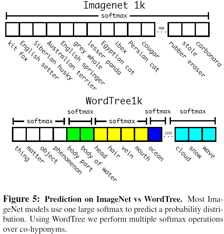
To validate this approach we train the Darknet-19 model on WordTree built using the 1000 class ImageNet. To build WordTree 1k we add in all of the intermediate nodes which expands the label space from 1000 to 1369. During training we propagate ground truth labels up the tree so that if an image is labelled as a “Norfolk terrier” it also gets labelled as a “dog” and a “mammal”, etc. To compute the conditional probabilities our model predicts a vector of 1369 values and we compute the softmax over all sysnsets that are hyponyms of the same concept, see Figure 5.

为了验证这种方法，我们在使用 1000 类 ImageNet 建立的 WordTree 上训练 Darknet-19 模型。为了构建 WordTree 1k，我们添加了所有中间节点，从而将标签空间从 1000 个扩展到 1369 个。在训练过程中，我们会将 ground truth 标签向树上传播，因此如果一张图片被标记为 “Norfolk terrier”，它也会被标记为 "dog "和 "mammal "等。为了计算条件概率，我们的模型预测了一个包含 1369 个值的向量，并计算了同一概念的所有系统集的软最大值（softmax），见图 5。

Using the same training parameters as before, our hierarchical Darknet-19 achieves 71.9% top-1 accuracy and 90.4% top-5 accuracy. Despite adding 369 additional concepts and having our network predict a tree structure our accuracy only drops marginally. Performing classification in this manner also has some benefits. Performance degrades gracefully on new or unknown object categories. For example, if the network sees a picture of a dog but is uncertain what type of dog it is, it will still predict “dog” with high confidence but have lower confidences spread out among the hyponyms.

使用与之前相同的训练参数，我们的分层 Darknet-19 实现了 71.9% 的 top-1 准确率和 90.4% 的 top-5 准确率。尽管增加了 369 个概念并让网络预测树状结构，但我们的准确率仅略有下降。以这种方式进行分类也有一些好处。在出现新的或未知的对象类别时，性能会从容下降。例如，如果网络看到一张狗的图片，但不确定它是什么类型的狗，那么它仍然会以较高的置信度预测 “狗”，但其较低的置信度会分散到各个假名中。

This formulation also works for detection. Now, instead of assuming every image has an object, we use YOLOv2’s objectness predictor to give us the value of Pr(physical object). The detector predicts a bounding box and the tree of probabilities. We traverse the tree down, taking the highest confidence path at every split until we reach some threshold and we predict that object class.

这种方法同样适用于检测。现在，我们不再假设每张图像都有一个物体，而是使用 YOLOv2 的物体性预测器来给出 Pr(physical object)值。检测器会预测一个边界框和概率树。我们沿着概率树向下遍历，在每次分割时选择置信度最高的路径，直到达到某个阈值并预测出该物体类别。

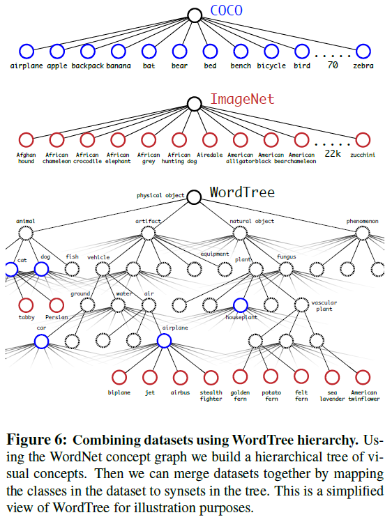
Dataset combination with WordTree. We can use WordTree to combine multiple datasets together in a sensible fashion. We simply map the categories in the datasets to synsets in the tree. Figure 6 shows an example of using WordTree to combine the labels from ImageNet and COCO. WordNet is extremely diverse so we can use this technique with most datasets.

用 WordTree 组合数据集。我们可以使用 WordTree 以合理的方式将多个数据集组合在一起。我们只需将数据集中的类别映射到树中的同义词集。图 6 显示了使用 WordTree 将 ImageNet 和 COCO 的标签组合在一起的示例。WordNet 种类繁多，因此我们可以在大多数数据集上使用这种技术。

Joint classification and detection. Now that we can combine datasets using WordTree we can train our joint model on classification and detection. We want to train an extremely large scale detector so we create our combined dataset using the COCO detection dataset and the top 9000 classes from the full ImageNet release. We also need to evaluate our method so we add in any classes from the ImageNet detection challenge that were not already included. The corresponding WordTree for this dataset has 9418 classes. ImageNet is a much larger dataset so we balance the dataset by oversampling COCO so that ImageNet is only larger by a factor of 4:1.

联合分类和检测。既然我们可以使用 WordTree 来组合数据集，我们就可以训练分类和检测联合模型。我们希望训练一个超大规模的检测器，因此我们使用 COCO 检测数据集和完整 ImageNet 版本中的前 9000 个类别创建了联合数据集。我们还需要评估我们的方法，因此我们添加了 ImageNet 检测挑战赛中尚未包含的任何类别。该数据集对应的 WordTree 有 9418 个类别。ImageNet 是一个更大的数据集，因此我们通过对 COCO 进行超采样来平衡数据集，这样 ImageNet 只比 COCO 大 4:1。

Using this dataset we train YOLO9000. We use the base YOLOv2 architecture but only 3 priors instead of 5 to limit the output size. When our network sees a detection image we backpropagate loss as normal. For classification loss, we only backpropagate loss at or above the corresponding level of the label. For example, if the label is “dog” we do assign any error to predictions further down in the tree, “German Shepherd” versus “Golden Retriever”, because we do not have that information.

我们使用该数据集训练 YOLO9000。我们使用基本的 YOLOv2 架构，但只有 3 个前验而不是 5 个前验，以限制输出大小。当我们的网络看到检测图像时，我们会像往常一样反向传播损失。对于分类损失，我们只反向传播标签相应级别或以上的损失。例如，如果标签是 “dog”，我们不会将任何误差分配给树中更下一级的预测，如 "German Shepherd "和 “Golden Retriever”，因为我们没有这些信息。

When it sees a classification image we only backpropagate classification loss. To do this we simply find the bounding box that predicts the highest probability for that class and we compute the loss on just its predicted tree. We also assume that the predicted box overlaps what would be the ground truth label by at least .3 IOU and we backpropagate objectness loss based on this assumption.

当看到分类图像时，我们只反向传播分类损失。为此，我们只需找到预测该类概率最高的预测框，然后只计算其预测树上的损失。我们还假设预测框与地面实况标签重叠至少 0.3 IOU，并根据这一假设反向传播对象损失。

Using this joint training, YOLO9000 learns to find objects in images using the detection data in COCO and it learns to classify a wide variety of these objects using data from ImageNet.

通过这种联合训练，YOLO9000 学会了使用 COCO 中的检测数据查找图像中的目标，并学会了使用 ImageNet 中的数据对这些目标进行分类。

We evaluate YOLO9000 on the ImageNet detection task. The detection task for ImageNet shares on 44 object categories with COCO which means that YOLO9000 has only seen classification data for the majority of the test categories. YOLO9000 gets 19.7 mAP overall with 16.0 mAP on the disjoint 156 object classes that it has never seen any labelled detection data for. This mAP is higher than results achieved by DPM but YOLO9000 is trained on different datasets with only partial supervision [4]. It also is simultaneously detecting 9000 other categories, all in real-time.

我们在 ImageNet 检测任务中对 YOLO9000 进行了评估。ImageNet 的检测任务与 COCO 共享 44 个对象类别，这意味着 YOLO9000 只看到了大部分检测类别的分类数据。YOLO9000 的总体 mAP 为 19.7，在从未见过任何标记检测数据的 156 个不相连的对象类别上的 mAP 为 16.0。这一 mAP 高于 DPM 的结果，但 YOLO9000 是在不同的数据集上训练的，只有部分监督[4]。此外，YOLO9000 还同时实时检测 9000 个其他类别。

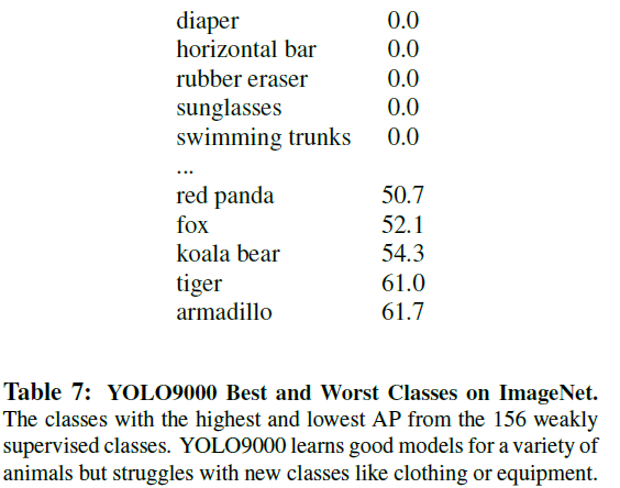
YOLO9000 learns new species of animals well but struggles with learning categories like clothing and equipment. New animals are easier to learn because the objectness predictions generalize well from the animals in COCO. Conversely, COCO does not have bounding box label for any type of clothing, only for person, so YOLO9000 struggles to model categories like “sunglasses” or “swimming trunks”.

YOLO9000 能很好地学习新的动物种类，但在学习服装和设备等类别时却很吃力。新动物比较容易学习，因为 COCO 中的对象性预测可以很好地概括动物。相反，COCO 没有为任何类型的服装（只有人）提供边界框标签，因此 YOLO9000 在为 "太阳镜 "或 "泳裤 "等类别建模时很吃力。

5 Conclusion

We introduce YOLOv2 and YOLO9000, real-time detection systems. YOLOv2 is state-of-the-art and faster than other detection systems across a variety of detection datasets. Furthermore, it can be run at a variety of image sizes to provide a smooth tradeoff between speed and accuracy.

我们介绍实时检测系统 YOLOv2 和 YOLO9000。YOLOv2 是目前最先进的检测系统，在各种检测数据集上都比其他检测系统更快。此外，它还可以在各种图像尺寸下运行，从而在速度和准确性之间实现平稳权衡。

YOLO9000 is a real-time framework for detection more than 9000 object categories by jointly optimizing detection and classification. We use WordTree to combine data from various sources and our joint optimization technique to train simultaneously on ImageNet and COCO. YOLO9000 is a strong step towards closing the dataset size gap between detection and classification.

YOLO9000 是一个通过联合优化检测和分类来检测 9000 多个目标类别的实时框架。我们使用 WordTree 将不同来源的数据结合起来，并使用我们的联合优化技术同时在 ImageNet 和 COCO 上进行训练。YOLO9000 在缩小检测和分类之间的数据集规模差距方面迈出了坚实的一步。

Many of our techniques generalize outside of object detection. Our WordTree representation of ImageNet offers a richer, more detailed output space for image classification. Dataset combination using hierarchical classification would be useful in the classification and segmentation domains. Training techniques like multi-scale training could provide benefit across a variety of visual tasks.

我们的许多技术都可用于目标检测以外的领域。我们的 ImageNet WordTree 表示法为图像分类提供了更丰富、更详细的输出空间。在分类和分割领域，使用分层分类的数据集组合将非常有用。多尺度训练等训练技术可为各种视觉任务带来益处。

For future work we hope to use similar techniques for weakly supervised image segmentation. We also plan to improve our detection results using more powerful matching strategies for assigning weak labels to classification data during training. Computer vision is blessed with an enormous amount of labelled data. We will continue looking for ways to bring different sources and structures of data together to make stronger models of the visual world.

在未来的工作中，我们希望将类似的技术用于弱监督图像分割。我们还计划在训练过程中使用更强大的匹配策略为分类数据分配弱标签，从而改进我们的检测结果。计算机视觉拥有海量的标签数据。我们将继续寻找方法，将不同来源和结构的数据整合在一起，以建立更强大的视觉世界模型。

Acknowledgements: We would like to thank Junyuan Xie for helpful discussions about constructing WordTree. This work is in part supported by ONR N00014-13-1-0720, NSF IIS-1338054, NSF-1652052, NRI-1637479, Allen Distinguished Investigator Award, and the Allen Institute for Artificial Intelligence.

致谢： 感谢谢俊元就构建 WordTree 所做的有益讨论。这项工作部分得到了 ONR N00014-13-1-0720、NSF IIS-1338054、NSF-1652052、NRI-1637479、艾伦杰出研究员奖和艾伦人工智能研究所的支持。