spark mllib源码分析之DecisionTree与GBDT

相关文章 spark源码分析之随机森林(Random Forest)

我们在前面的文章讲过，在spark的实现中，树模型的依赖链是GBDT-> Decision Tree-> Random Forest，前面介绍了最基础的Random Forest的实现，在此基础上我们介绍Decision Tree和GBDT的实现。

1. Decision Tree

1.1. DT的使用

官方给出的demo

// Train a DecisionTree model.
    //  Empty categoricalFeaturesInfo indicates all features are continuous.
    val numClasses = 2
    val categoricalFeaturesInfo = Map[Int, Int]()
    val impurity = "gini"
    val maxDepth = 5
    val maxBins = 32

    val model = DecisionTree.trainClassifier(trainingData, numClasses, categoricalFeaturesInfo,
      impurity, maxDepth, maxBins)

其入参除了不需要指定树个数，其他参数与随机森林类似，不再赘述

1.2 实现

主要的逻辑在DecisionTree.scala的run函数中

  /**
   * Method to train a decision tree model over an RDD
   * @param input Training data: RDD of [[org.apache.spark.mllib.regression.LabeledPoint]]
   * @return DecisionTreeModel that can be used for prediction
   */
  @Since("1.2.0")
  def run(input: RDD[LabeledPoint]): DecisionTreeModel = {
    // Note: random seed will not be used since numTrees = 1.
    val rf = new RandomForest(strategy, numTrees = 1, featureSubsetStrategy = "all", seed = 0)
    val rfModel = rf.run(input)
    rfModel.trees(0)
  }

其实就是Random Forest 1棵树的情形，同时特征不再抽样。

2. Gradient Boosting Decision Tree

2.1. 算法简介

简称GBDT，中文译作梯度提升决策树，估计没几个人听过。这里贴几张之前介绍GBDT的PPT，简单回顾起算法原理，其中内容来自wikipedia和”From RankNet to LambdaRank to LambdaMAR An Overview”这篇文章。

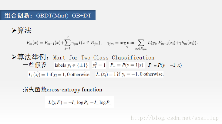
2.1.1. 算法原理

在这个算法里面，并没有限定使用决策树，如果使用决策树，对应里面的h应该是树结构，我们以决策树说明
1. 使用原始样本直接训练一棵树
循环训练
2. 计算伪残差，实际是梯度
3. 将2中的伪残差作为样本的label去训练决策树
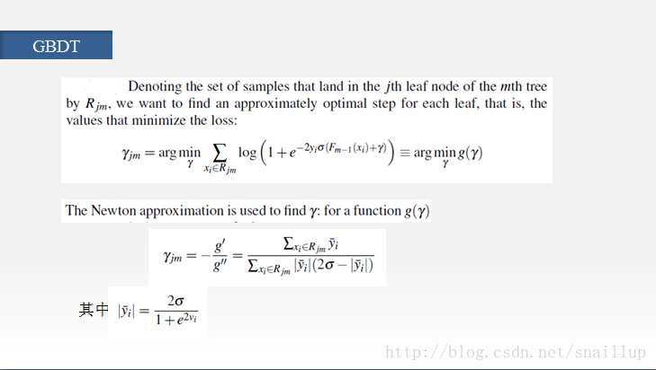
4. 这里是用最优化方法计算叶子节点的输出，而spark中直接使用的均值
5. 计算当轮模型的输出，方法是上一轮的输出加上本轮的预测值
6. 循环结束后，输出模型

2.1.2. 以二分类为例

2.2. GBDT使用

官方demo

// Train a GradientBoostedTrees model.
// The defaultParams for Classification use LogLoss by default.
val boostingStrategy = BoostingStrategy.defaultParams("Classification")
boostingStrategy.numIterations = 3 // Note: Use more iterations in practice.
boostingStrategy.treeStrategy.numClasses = 2
boostingStrategy.treeStrategy.maxDepth = 5
// Empty categoricalFeaturesInfo indicates all features are continuous.
boostingStrategy.treeStrategy.categoricalFeaturesInfo = Map[Int, Int]()

val model = GradientBoostedTrees.train(trainingData, boostingStrategy)

首先初始化训练参数boostingStrategy，然后设置其迭代次数，分类树，树的最大深度，离散特征及其特征值数，我们看下默认的参数都有哪些

/**
   * Returns default configuration for the boosting algorithm
   * @param algo Learning goal.  Supported:
   *             [[org.apache.spark.mllib.tree.configuration.Algo.Classification]],
   *             [[org.apache.spark.mllib.tree.configuration.Algo.Regression]]
   * @return Configuration for boosting algorithm
   */
  @Since("1.3.0")
  def defaultParams(algo: Algo): BoostingStrategy = {
    val treeStrategy = Strategy.defaultStrategy(algo)
    treeStrategy.maxDepth = 3
    algo match {
      case Algo.Classification =>
        treeStrategy.numClasses = 2
        new BoostingStrategy(treeStrategy, LogLoss)
      case Algo.Regression =>
        new BoostingStrategy(treeStrategy, SquaredError)
      case _ =>
        throw new IllegalArgumentException(s"$algo is not supported by boosting.")
    }
  }

默认树的最大深度为3，如果是分类，为二分类，使用LogLoss；如果是回归，使用SquareError，均方误差。然后使用Strategy的默认参数

  /**
   * Construct a default set of parameters for [[org.apache.spark.mllib.tree.DecisionTree]]
   * @param algo Algo.Classification or Algo.Regression
   */
  @Since("1.3.0")
  def defaultStrategy(algo: Algo): Strategy = algo match {
    case Algo.Classification =>
      new Strategy(algo = Classification, impurity = Gini, maxDepth = 10,
        numClasses = 2)
    case Algo.Regression =>
      new Strategy(algo = Regression, impurity = Variance, maxDepth = 10,
        numClasses = 0)
  }

Strategy的默认参数也比较简单，其意义参见之前的文章。

2.3. GBDT实现

其实现开始于GradientBoostedTrees.scala的run函数

  /**
   * Method to train a gradient boosting model
   * @param input Training dataset: RDD of [[org.apache.spark.mllib.regression.LabeledPoint]].
   * @return a gradient boosted trees model that can be used for prediction
   */
  @Since("1.2.0")
  def run(input: RDD[LabeledPoint]): GradientBoostedTreesModel = {
    val algo = boostingStrategy.treeStrategy.algo
    algo match {
      case Regression =>
        GradientBoostedTrees.boost(input, input, boostingStrategy, validate = false)
      case Classification =>
        // Map labels to -1, +1 so binary classification can be treated as regression.
        val remappedInput = input.map(x => new LabeledPoint((x.label * 2) - 1, x.features))
        GradientBoostedTrees.boost(remappedInput, remappedInput, boostingStrategy, validate = false)
      case _ =>
        throw new IllegalArgumentException(s"$algo is not supported by the gradient boosting.")
    }
  }

从其注释可以看到，spark GBDT只实现了二分类，并且二分类的class必须是0/1，其把0/1转化成-1/+1的label，然后按回归处理。

2.3.2. 数据结构

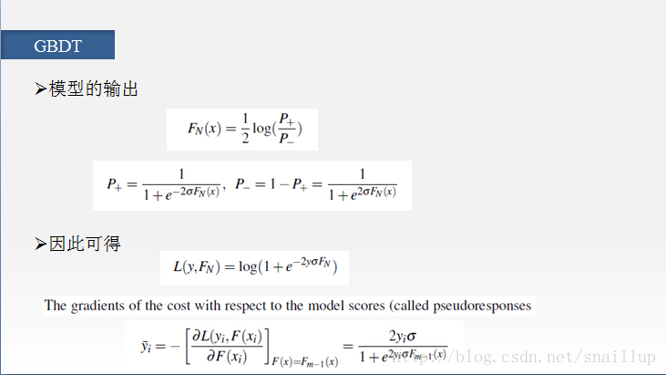
2.3.2.1. LogLoss

在第二页PPT中我们给出了loss，spark使用的loss是σ=1，log前增加了系数2的情况

$$L(y,F_N)=2log(1+e^{-2yF_N})$$
对应梯度变成

$$g=4y/(1+e^{2yF_{m-1}(x)})$$
其中m-1指的是在第m次迭代中，使用的是m-1次的预测值。注意到我们的PPT的第四页的γ，其实是叶子节点的预测值，是通过最优化得到的，而spark这里使用的是Random Forest的代码，其impurity选择的是variance，因此预测值是均值。

  @Since("1.2.0")
  override def gradient(prediction: Double, label: Double): Double = {
    - 4.0 * label / (1.0 + math.exp(2.0 * label * prediction))
  }

  override private[mllib] def computeError(prediction: Double, label: Double): Double = {
  //loss
    val margin = 2.0 * label * prediction
    // The following is equivalent to 2.0 * log(1 + exp(-margin)) but more numerically stable.
    2.0 * MLUtils.log1pExp(-margin)
  }

SquaredError比较简单，这里不再啰嗦了。

2.3.1. init

将传入的参数转成训练时的参数，cache predError和validatePredError，并且按treeStrategy.getCheckpointInterval（default 10）建立checkpoint。这里代码比较简单，不再赘述。

2.3.2. build the first tree

参照算法原理的第一步，训练了第一棵树，并且将weight设为1，，然后计算错误率。调用了computeInitialPredictionAndError函数

  /**
   * :: DeveloperApi ::
   * Compute the initial predictions and errors for a dataset for the first
   * iteration of gradient boosting.
   * @param data: training data.
   * @param initTreeWeight: learning rate assigned to the first tree.
   * @param initTree: first DecisionTreeModel.
   * @param loss: evaluation metric.
   * @return a RDD with each element being a zip of the prediction and error
   *         corresponding to every sample.
   */
  @Since("1.4.0")
  @DeveloperApi
  def computeInitialPredictionAndError(
      data: RDD[LabeledPoint],
      initTreeWeight: Double,
      initTree: DecisionTreeModel,
      loss: Loss): RDD[(Double, Double)] = {
    data.map { lp =>
      val pred = initTreeWeight * initTree.predict(lp.features)
      val error = loss.computeError(pred, lp.label)
      (pred, error)
    }
  }

其中预测值直接使用DT的predict来预测，error使用loss的computeError函数，我们上面有介绍。

2.3.3. 循环训练

2.3.3.1. 样本处理

对应算法的第2步，计算梯度，并且作为label更新样本

val data = predError.zip(input).map { case ((pred, _), point) =>
        LabeledPoint(-loss.gradient(pred, point.label), point.features)
      }

2.3.3.2. 训练树

对应算法的第3和第4步，用第2步的样本作为输入，训练决策树

val model = new DecisionTree(treeStrategy).run(data)
timer.stop(s"building tree $m")
// Update partial model
baseLearners(m) = model
// Note: The setting of baseLearnerWeights is incorrect for losses other than SquaredError.
//       Technically, the weight should be optimized for the particular loss.
//       However, the behavior should be reasonable, though not optimal.
baseLearnerWeights(m) = learningRate

2.3.3.3. 计算模型输出

实际调用updatePredictionError函数，入参是原始的样本，上一轮的错误率（实际包含上一轮的模型输出），本来的决策树，学习率和loss计算对象。

  /**
   * :: DeveloperApi ::
   * Update a zipped predictionError RDD
   * (as obtained with computeInitialPredictionAndError)
   * @param data: training data.
   * @param predictionAndError: predictionError RDD
   * @param treeWeight: Learning rate.
   * @param tree: Tree using which the prediction and error should be updated.
   * @param loss: evaluation metric.
   * @return a RDD with each element being a zip of the prediction and error
   *         corresponding to each sample.
   */
  @Since("1.4.0")
  @DeveloperApi
  def updatePredictionError(
    data: RDD[LabeledPoint],
    predictionAndError: RDD[(Double, Double)],
    treeWeight: Double,
    tree: DecisionTreeModel,
    loss: Loss): RDD[(Double, Double)] = {

    val newPredError = data.zip(predictionAndError).mapPartitions { iter =>
      iter.map { case (lp, (pred, error)) =>
      //计算本轮模型的预测值
        val newPred = pred + tree.predict(lp.features) * treeWeight
        //计算本轮误差
        val newError = loss.computeError(newPred, lp.label)
        //newPred是累计，包含至本轮的模型输出
        (newPred, newError)
      }
    }
    newPredError
  }

代码中使用到的函数我们之前都有介绍。

2.3.3.3. validation(early stop)

类似计算错误率，只是样本使用validationInput，看平均误差是否减少，如果不能使误差减小就结束训练，相当于出现过拟合了；如果能，就继续训练，并且记录最好的模型的index。这里一次误差变大就结束训练比较武断，最好应该有一定的阈值，避免单次训练的波动。代码比较简单，就不放了。

2.3.3.4. 训练收尾

训练完成后，根据记录的最优模型的index，构造GradientBoostedTreesModel。

3.结语

从上面的分析可以看到，由于spark在Random Forest特征方面的限制，以及GBDT实现中直接使用均值作为叶子节点的输出值，early stop等，spark在树模型上的精度可能会差一点，实际使用的话，最好与其他实现比较后决定是否使用。