机器学习笔记——逻辑斯蒂回归

参数化模型与非参数化

像前面的KNN模型，不需要对f的形式做出假设，在学习中可以得到任意的模型叫非参数化
而需要对参数进行学习的模型叫参数化模型，参数化限制了f的可能的集合，学习难度相对较低

逻辑斯蒂回归

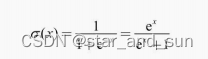
逻辑斯蒂函数

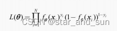
似然函数

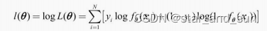
对数似然函数

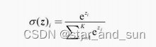
在多分类使用softmax函数


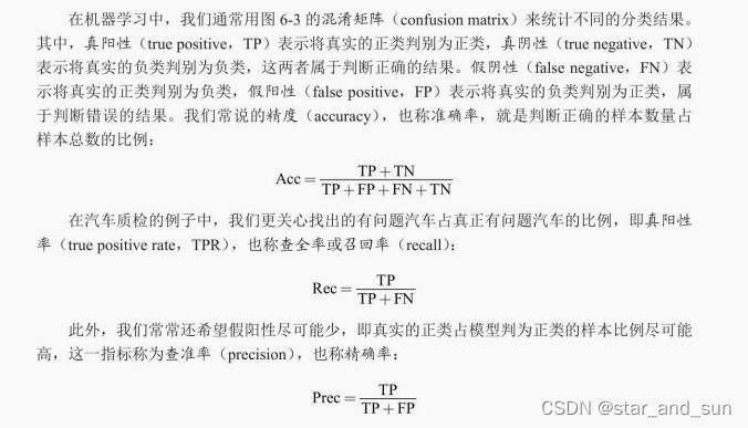
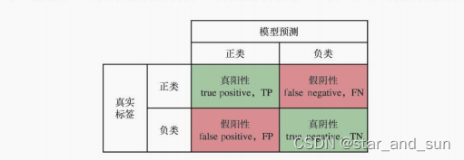
重点

ROC曲线

真阳性率 、假阳性率 FPR的变化曲线就叫做ROC曲线
ROC曲线的面积就叫AUC

import numpy as np
import matplotlib.pyplot as plt
from matplotlib.ticker import MaxNLocator
#%%
# 从源文件中读入数据并处理
lines = np.loadtxt('./data/lr_dataset.csv', delimiter=',', dtype=float)
x_total = lines[:, 0:2]
y_total = lines[:, 2]
print('数据集大小：', len(x_total))
#%%
pos_index=np.where(y_total==1)
neg_index=np.where(y_total==0)
plt.scatter(x_total[pos_index,0],x_total[pos_index,1],marker='o',color='coral',s=10)
plt.scatter(x_total[neg_index,0],x_total[neg_index,1],marker='x',color='blue',s=10)
plt.xlabel('X1')
plt.ylabel('X2')
plt.show()

#%%
np.random.seed(0)
ratio = 0.7
split = int(len(x_total) * ratio)
idx = np.random.permutation(len(x_total))
x_total = x_total[idx]
y_total = y_total[idx]
x_train, y_train = x_total[:split], y_total[:split]
x_test, y_test = x_total[split:], y_total[split:]

#%%
y_test
idx=np.argsort(y_test[::-1])

#%%
y_test
#%%
def acc(y_true,y_pred):
    return np.mean(y_true==y_pred)
def auc(y_true,y_pred):
    idx=np.argsort(y_pred)[::-1]
    y_true=y_true[idx]
    y_pred=y_pred[idx]
    tp=np.cumsum(y_true) #累加
    fp=np.cumsum(1-y_true)
    tpr=tp/tp[-1]
    fpr=fp/fp[-1]
    s=0.0
    tpr = np.concatenate([[0], tpr]) #拼接函数
    fpr = np.concatenate([[0], fpr])
    for i in range(1, len(fpr)):
        s += (fpr[i] - fpr[i - 1]) * tpr[i]
        return s
#%%

def logistic(z):
    return 1/(1+np.exp(-z))
def GD(num_steps,learning_rate,l2_coef):
    theta=np.random.normal(size=(X.shape[1],))
    train_losses=[]
    test_losses = []
    train_acc = []
    test_acc = []
    train_auc = []
    test_auc = []
    for i in range(num_steps):
        pred = logistic(X @ theta)
        grad = -X.T @ (y_train - pred) + l2_coef * theta
        theta -= learning_rate * grad
        train_loss = - y_train.T @ np.log(pred) \
                     - (1 - y_train).T @ np.log(1 - pred) \
                     + l2_coef * np.linalg.norm(theta) ** 2 / 2
        train_losses.append(train_loss / len(X))
        test_pred = logistic(X_test @ theta)
        test_loss = - y_test.T @ np.log(test_pred) \
                    - (1 - y_test).T @ np.log(1 - test_pred)
        test_losses.append(test_loss / len(X_test))
        # 记录各个评价指标，阈值采用0.5
        train_acc.append(acc(y_train, pred >= 0.5))
        test_acc.append(acc(y_test, test_pred >= 0.5))
        train_auc.append(auc(y_train, pred))
        test_auc.append(auc(y_test, test_pred))
    return theta, train_losses, test_losses, \
    train_acc, test_acc, train_auc, test_auc
#%%
# 定义梯度下降迭代的次数，学习率，以及L2正则系数
num_steps = 250
learning_rate = 0.002
l2_coef = 1.0
np.random.seed(0)

# 在x矩阵上拼接1
X = np.concatenate([x_train, np.ones((x_train.shape[0], 1))], axis=1)
X_test = np.concatenate([x_test, np.ones((x_test.shape[0], 1))], axis=1)

theta, train_losses, test_losses, train_acc, test_acc, \
    train_auc, test_auc = GD(num_steps, learning_rate, l2_coef)

# 计算测试集上的预测准确率
y_pred = np.where(logistic(X_test @ theta) >= 0.5, 1, 0)
final_acc = acc(y_test, y_pred)
print('预测准确率：', final_acc)
print('回归系数：', theta)

plt.figure(figsize=(13, 9))
xticks = np.arange(num_steps) + 1


#%%
# 绘制训练曲线
plt.subplot(221)
plt.plot(xticks, train_losses, color='blue', label='train loss')
plt.plot(xticks, test_losses, color='red', ls='--', label='test loss')
plt.gca().xaxis.set_major_locator(MaxNLocator(integer=True))
plt.xlabel('Epochs')
plt.ylabel('Loss')
plt.legend()

#%%
# 绘制准确率
plt.subplot(222)
plt.plot(xticks, train_acc, color='blue', label='train accuracy')
plt.plot(xticks, test_acc, color='red', ls='--', label='test accuracy')
plt.gca().xaxis.set_major_locator(MaxNLocator(integer=True))
plt.xlabel('Epochs')
plt.ylabel('Accuracy')
plt.legend()