DataScience_笔记_7

1. Classifier: K-Nearest Neighbors

代码实例：

用KNN算法处理 MNIST 数据集中的手写数字图像：
MINIST.py

import numpy as np
from urllib import request
import gzip
import pickle

filename = [
["training_images","train-images-idx3-ubyte.gz"],
["test_images","t10k-images-idx3-ubyte.gz"],
["training_labels","train-labels-idx1-ubyte.gz"],
["test_labels","t10k-labels-idx1-ubyte.gz"]
]

def download_mnist():
    base_url = "http://yann.lecun.com/exdb/mnist/"
    for name in filename:
        print("Downloading "+name[1]+"...")
        request.urlretrieve(base_url+name[1], name[1])
    print("Download complete.")

def save_mnist():
    mnist = {}
    for name in filename[:2]:
        with gzip.open(name[1], 'rb') as f:
            mnist[name[0]] = np.frombuffer(f.read(), np.uint8, offset=16).reshape(-1,28*28)
    for name in filename[-2:]:
        with gzip.open(name[1], 'rb') as f:
            mnist[name[0]] = np.frombuffer(f.read(), np.uint8, offset=8)
    with open("mnist.pkl", 'wb') as f:
        pickle.dump(mnist,f)
    print("Save complete.")

def init():
    download_mnist()
    save_mnist()

def load():
    with open("mnist.pkl",'rb') as f:
        mnist = pickle.load(f)
    return mnist["training_images"], mnist["training_labels"], mnist["test_images"], mnist["test_labels"]

if __name__ == '__main__':
    init()

KNN_MINIST.py

import MINIST
from sklearn.neighbors import KNeighborsClassifier
import numpy as np

# MINIST.init()

# Load the MNIST data
train_data, train_label, test_data, test_label = MINIST.load()

# Normalize the data (Scale pixel values to [0, 1])
train_data = train_data.astype(np.float32) / 255.0
test_data = test_data.astype(np.float32) / 255.0

# Using kNN with 3 neighbors for now (you can tune this parameter)
neigh = KNeighborsClassifier(n_neighbors=3)
neigh.fit(train_data, train_label)

# 测试数据，用训练好的模型去测试test_data
# pred_labels = neigh.predict(test_data)
# print(sum(pred_labels==test_label)/test_label.shape[0])



from PIL import Image
# Load the image using PIL
img = Image.open('input_number_picture.png').convert("L")

# Resize to suitable
img = img.resize((28, 28), Image.LANCZOS)

# Convert the PIL image to a NumPy array
image = np.array(img)

# Binarization
threshold = 200
image[image >= threshold] = 255
image[image < threshold] = 0
image = 255 - image

# Normalize (scale values to [0, 1])
image = image.astype(np.float32) / 255.0

processed_image = image.reshape([1, -1])
pred_label = neigh.predict(processed_image)
print(pred_label)

I_image = Image.fromarray((processed_image.reshape(28, 28) * 255).astype(np.uint8))
I_image.save("output_number_picture.png")

2. Classifier: Decision Tree

优点：

1. 直观且易于解释: 与其他机器学习算法相比，决策树的结果是可视化的，并且直观容易理解，这使得它非常适合在需要解释模型决策过程的场景中使用。
2. 不需要数据预处理: 决策树不需要特征标准化或规范化，而且它们可以处理数值型和分类数据。
3. 特征选择: 决策树可以进行自动的特征选择，并且可以显示每个特征的相对重要性。
4. 可以处理非线性关系: 决策树能够捕获数据中的非线性关系，不需要事先进行数据转换。
5. 不需要任何假设: 决策树不需要对数据分布做出任何假设，这与例如线性回归等方法形成对比。
6. 快速: 用于训练和预测的决策树算法通常很快。
7. 能够处理缺失值: 一些决策树算法（如C4.5）可以处理具有缺失值的数据。

缺点：

1. 容易过拟合: 尤其是当决策树深度很大时，它们很容易对数据进行过拟合。这可以通过设置树的最大深度或使用剪枝技术来缓解。
2. 不稳定性: 数据中的小变化可能导致生成一个完全不同的决策树。这可以通过使用集合方法，如随机森林来缓解。
3. 局部最优: 决策树的训练是基于贪婪算法的，这意味着它们可能会陷入局部最优而不是全局最优。
4. 对连续变量的处理: 当决策树对连续变量进行切分时，它可能不够精确，因为它使用阈值进行切分。
5. 可能不是最有效的: 对于某些复杂的问题，如图像和声音处理，决策树可能不是最有效的解决方案。在这些情况下，其他算法（如深度学习模型）可能更为适用。

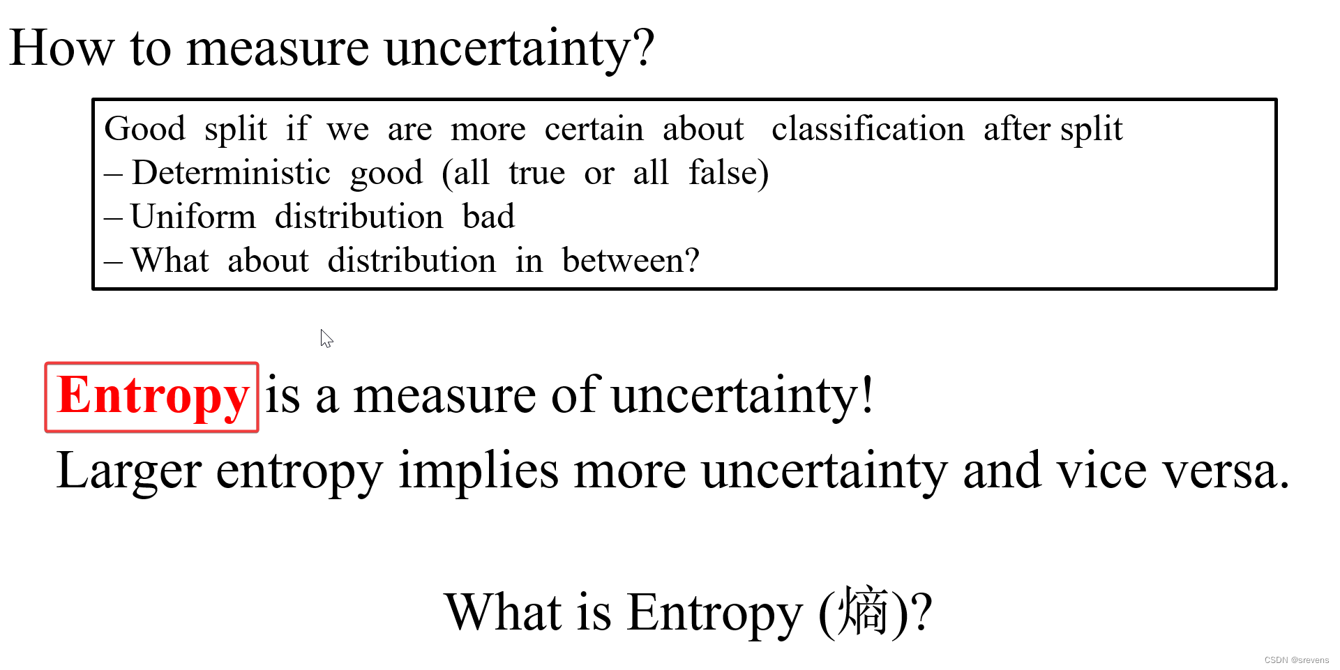
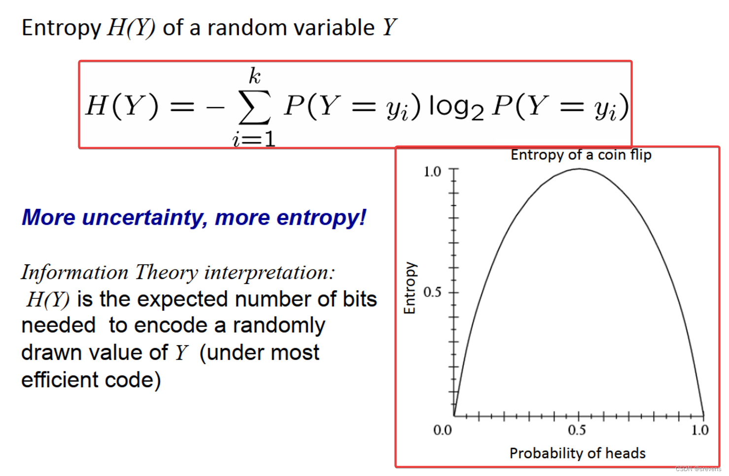
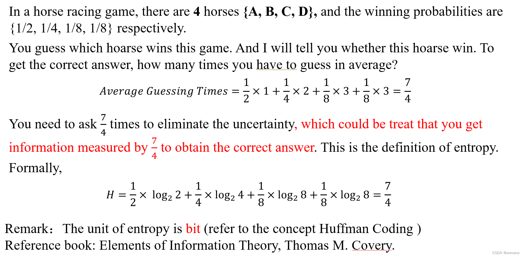
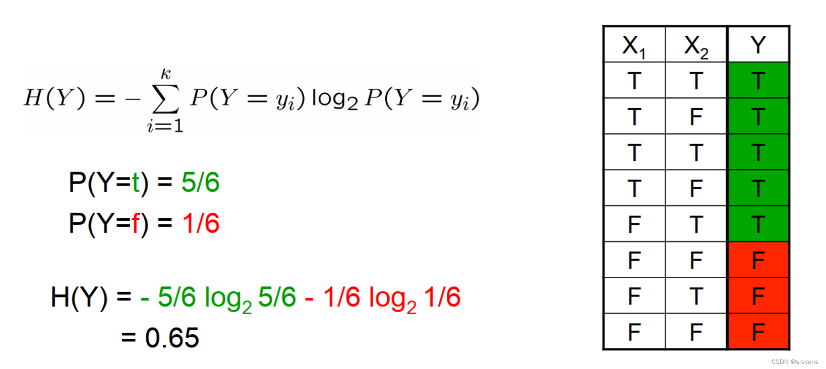
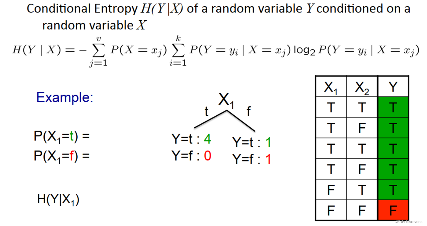
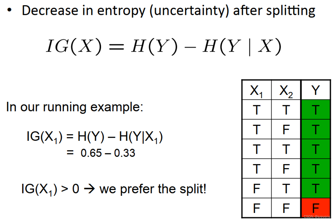
熵的定义