贷款违约预测学习笔记

最新推荐文章于 2023-12-28 06:59:46 发布

submarineas

最新推荐文章于 2023-12-28 06:59:46 发布

阅读量4.4k

点赞数 2

分类专栏：机器学习文章标签： python 机器学习数据分析

本文链接：https://blog.csdn.net/submarineas/article/details/108562718

版权

机器学习专栏收录该内容

25 篇文章 6 订阅

订阅专栏

赛题介绍

链接：https://tianchi.aliyun.com/competition/entrance/531830/information

赛题数据

赛题以预测用户贷款是否违约为任务，数据集报名后可见并可下载，该数据来自某信贷平台的贷款记录，总数据量超过120w，包含47列变量信息，其中15列为匿名变量。为了保证比赛的公平性，将会从中抽取80万条作为训练集，20万条作为测试集A，20万条作为测试集B，同时会对employmentTitle、purpose、postCode和title等信息进行脱敏。
在这里插入图片描述

这是直接打开Excel后经过粗略判断画的一个图，详细信息后面会根据后续的describe() 和 info做进一步优化，通过思维导图的方式更有利于熟悉数据，也便于之后得到自动划分后的数据做主观判断。但可惜我忘记了现在xmind好像没有经过破解，很多功能用不了，比如链接两个子分支的框没法画，还有就是标注给的不是特别多，不然就选择processon了。

评测标准

提交结果为每个测试样本是1的概率，也就是y为1的概率。评价方法为AUC评估模型效果（越大越好）。

数据处理

导入数据

先导入大致需要用到的包，编程环境为Windows，代码为：

import pandas as pd
import numpy as np
import matplotlib.pyplot as plt 
import seaborn as sns
from sklearn.preprocessing import OneHotEncoder, LabelEncoder

import sys
import warnings

if not sys.warnoptions:
    warnings.simplefilter("ignore")

from IPython.core.interactiveshell import InteractiveShell
"""
win下显示所有结果与中文
"""
InteractiveShell.ast_node_interactivity = "all"
plt.rcParams['font.sans-serif']=['SimHei']
plt.rcParams['axes.unicode_minus']=False

然后导入本次比赛的数据与初步分析：

# 导入数据
train = pd.read_csv('train.csv',index_col='id')
testA = pd.read_csv('testA.csv',index_col='id')
data = pd.concat([train, testA], axis=0, ignore_index=True)
testA.shape		# (800000, 47)
train.shape		# (200000, 48)
train.info()

"""
<class 'pandas.core.frame.DataFrame'>
RangeIndex: 800000 entries, 0 to 799999
Data columns (total 47 columns):
 #   Column              Non-Null Count   Dtype  
---  ------              --------------   -----  
 0   id                  800000 non-null  int64  
 1   loanAmnt            800000 non-null  float64
 2   term                800000 non-null  int64  
 3   interestRate        800000 non-null  float64
 4   installment         800000 non-null  float64
 5   grade               800000 non-null  object 
 6   subGrade            800000 non-null  object 
 7   employmentTitle     799999 non-null  float64
 8   employmentLength    753201 non-null  object 
 9   homeOwnership       800000 non-null  int64  
 10  annualIncome        800000 non-null  float64
 11  verificationStatus  800000 non-null  int64  
 12  issueDate           800000 non-null  object 
 13  isDefault           800000 non-null  int64  
 14  purpose             800000 non-null  int64  
 15  postCode            799999 non-null  float64
 16  regionCode          800000 non-null  int64  
 17  dti                 799761 non-null  float64
 18  delinquency_2years  800000 non-null  float64
 19  ficoRangeLow        800000 non-null  float64
 20  ficoRangeHigh       800000 non-null  float64
 21  openAcc             800000 non-null  float64
 22  pubRec              800000 non-null  float64
 23  pubRecBankruptcies  799595 non-null  float64
 24  revolBal            800000 non-null  float64
 25  revolUtil           799469 non-null  float64
 26  totalAcc            800000 non-null  float64
 27  initialListStatus   800000 non-null  int64  
 28  applicationType     800000 non-null  int64  
 29  earliesCreditLine   800000 non-null  object 
 30  title               799999 non-null  float64
 31  policyCode          800000 non-null  float64
 32  n0                  759730 non-null  float64
 33  n1                  759730 non-null  float64
 34  n2                  759730 non-null  float64
 35  n2.1                759730 non-null  float64
 36  n4                  766761 non-null  float64
 37  n5                  759730 non-null  float64
 38  n6                  759730 non-null  float64
 39  n7                  759730 non-null  float64
 40  n8                  759729 non-null  float64
 41  n9                  759730 non-null  float64
 42  n10                 766761 non-null  float64
 43  n11                 730248 non-null  float64
 44  n12                 759730 non-null  float64
 45  n13                 759730 non-null  float64
 46  n14                 759730 non-null  float64
dtypes: float64(33), int64(9), object(5)
memory usage: 286.9+ MB
"""

看来和想的差不多，总共有5个object对象，排除掉这五列，继续分析是否是连续：

#过滤数值型类别特征
def get_numerical_serial_fea(data,feas):
    numerical_serial_fea = []
    numerical_noserial_fea = []
    for fea in feas:
        temp = data[fea].nunique()
        if temp <= 10:
            numerical_noserial_fea.append(fea)
            continue
        numerical_serial_fea.append(fea)
    return numerical_serial_fea,numerical_noserial_fea

numerical_fea = list(train.select_dtypes(exclude=['object']).columns)
numerical_serial_fea,numerical_noserial_fea = get_numerical_serial_fea(data_train,numerical_fea)

print("numerical_serial_fea：",numerical_serial_fea)
print("numerical_noserial_fea：",numerical_noserial_fea)

"""
numerical_serial_fea： ['loanAmnt', 'interestRate', 'installment', 'employmentTitle', 'annualIncome', 'purpose', 'postCode', 'regionCode', 'dti', 'delinquency_2years', 'ficoRangeLow', 'ficoRangeHigh', 'openAcc', 'pubRec', 'pubRecBankruptcies', 'revolBal', 'revolUtil', 'totalAcc', 'title', 'n0', 'n1', 'n2', 'n2.1', 'n4', 'n5', 'n6', 'n7', 'n8', 'n9', 'n10', 'n13', 'n14']
numerical_noserial_fea： ['term', 'homeOwnership', 'verificationStatus', 'initialListStatus', 'applicationType', 'policyCode', 'n11', 'n12']
"""

那么画的思维导图与代码的出来的结果基本一致，除了n1-n14没有细分外，这里的数据从类别来讲也相对简单，可以将其分为三类，分别是离散数值、连续数值和对象，相比于其它数据还存在混合型特征和离散对象等，这里看起来并没有，那么就能接着进行数据分析了。

数据分析

train.describe(percentiles=[.1, .2, .3, .4, .5, .6, .7, .8, .9, .99])

在这里插入图片描述
从这里我们可以得到很多的信息比如：

贷款期限20%的人选择5年，80%选择三年
训练集上目标isdefault为9:1，即有一成的人出现违约，如果后期出现严重偏态，那可以考虑减少未出现违约的样本量
很多列的min都是0，不排除是缺失值或者存在0这个类别，
…

缺失值统计

# nan可视化
missing = train.isnull().sum()/len(train)
missing = missing[missing > 0]
missing.sort_values(inplace=True)
missing.plot.bar()

在这里插入图片描述
本来还想换一种用plotly_express画，但好像电脑里包环境有点问题了，按照报错装了一堆包如nbformat >= 4.2，requests还有plotly-orca等包还是没有成功显示，等之后有时间再做一下环境管理。

那就换一种，根据之前看鱼佬代码里有提过可视化方式：

stats = []
for col in train.columns:
    stats.append((col, train[col].nunique(), train[col].isnull().sum() * 100 / train.shape[0], train[col].value_counts(normalize=True, dropna=False).values[0] * 100, train[col].dtype))
    
stats_df = pd.DataFrame(stats, columns=['Feature', 'Unique_values', 'Percentage of missing values', 'Percentage of values in the biggest category', 'type'])
stats_df.sort_values('Percentage of missing values', ascending=False)[:23]

"""
Feature	Unique_values	Percentage of missing values	Percentage of values in the biggest category	type
43	n11	5	8.719000	91.210250	float64
8	employmentLength	11	5.849875	32.844125	object
40	n8	102	5.033875	5.601000	float64
39	n7	70	5.033750	10.416375	float64
33	n1	33	5.033750	20.376000	float64
34	n2	50	5.033750	14.651375	float64
35	n2.1	50	5.033750	14.651375	float64
37	n5	65	5.033750	9.572000	float64
38	n6	107	5.033750	8.086500	float64
46	n14	31	5.033750	23.437625	float64
41	n9	44	5.033750	14.766750	float64
44	n12	5	5.033750	94.664375	float64
45	n13	28	5.033750	89.516375	float64
32	n0	39	5.033750	72.428375	float64
36	n4	46	4.154875	16.816125	float64
42	n10	76	4.154875	8.502875	float64
25	revolUtil	1286	0.066375	0.521250	float64
23	pubRecBankruptcies	11	0.050625	87.509500	float64
17	dti	6321	0.029875	0.074125	float64
7	employmentTitle	248683	0.000125	6.393625	float64
30	title	39644	0.000125	49.166750	float64
15	postCode	932	0.000125	1.119500	float64
18	delinquency_2years	30	0.000000	80.714375	float64
"""

但从目前看来，缺失值都不是很多，而且0的类别不好区分，所以暂时不对这部分做处理，因为影响不大，对我后面模型来讲。

异常值统计

#每个数字特征得分布可视化
f = pd.melt(data_train, value_vars=numerical_serial_fea)
g = sns.FacetGrid(f, col="variable",  col_wrap=2, sharex=False, sharey=False)
g = g.map(sns.distplot, "value")

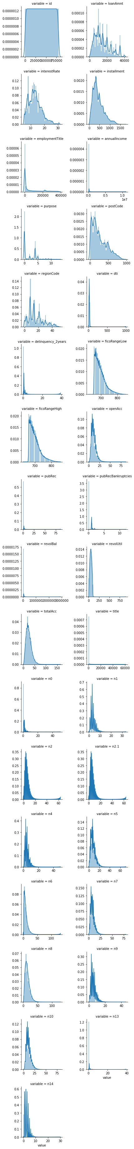
这里可以看到很多列都出现了偏态，我们可以挑出一列来看它的峰值：

print('峰度(Kurtosis): ', train['n0'].kurt())
print('偏度(Skewness): ', train['n0'].skew())
"""
峰度(Kurtosis):  46.53290236504996
偏度(Skewness):  5.1069085651560036
"""

数据分布情况

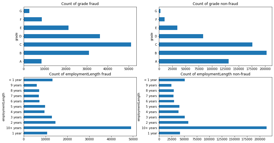
首先查看类别型变量在不同y值上的分布：

train_loan_fr = data_train.loc[data_train['isDefault'] == 1]
train_loan_nofr = data_train.loc[data_train['isDefault'] == 0]

fig, ((ax1, ax2), (ax3, ax4)) = plt.subplots(2, 2, figsize=(15, 8))
train_loan_fr.groupby('grade')['grade'].count().plot(kind='barh', ax=ax1, title='Count of grade fraud')
train_loan_nofr.groupby('grade')['grade'].count().plot(kind='barh', ax=ax2, title='Count of grade non-fraud')
train_loan_fr.groupby('employmentLength')['employmentLength'].count().plot(kind='barh', ax=ax3, title='Count of employmentLength fraud')
train_loan_nofr.groupby('employmentLength')['employmentLength'].count().plot(kind='barh', ax=ax4, title='Count of employmentLength non-fraud')
plt.show()

png

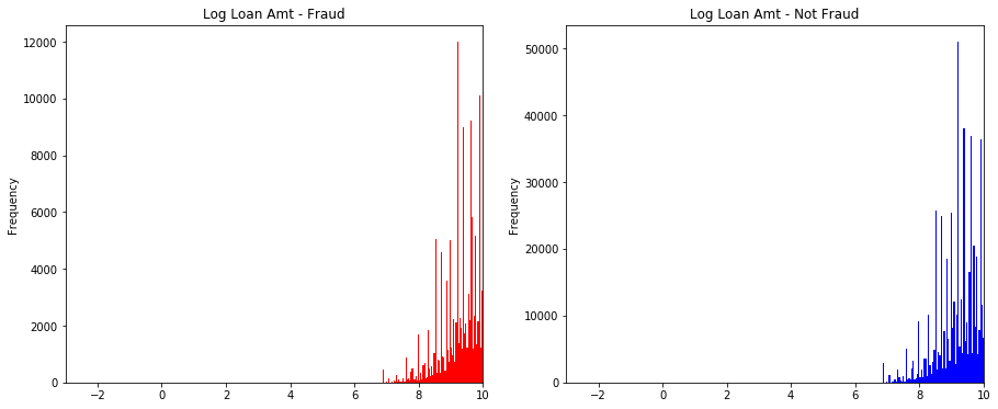
其次查看连续型变量在不同y值上的分布：

fig, ((ax1, ax2)) = plt.subplots(1, 2, figsize=(15, 6))
data_train.loc[data_train['isDefault'] == 1] \
    ['loanAmnt'].apply(np.log) \
    .plot(kind='hist',
          bins=100,
          title='Log Loan Amt - Fraud',
          color='r',
          xlim=(-3, 10),
         ax= ax1)
data_train.loc[data_train['isDefault'] == 0] \
    ['loanAmnt'].apply(np.log) \
    .plot(kind='hist',
          bins=100,
          title='Log Loan Amt - Not Fraud',
          color='b',
          xlim=(-3, 10),
         ax=ax2)

png

特征工程

处理缺失值和异常值，以及构建新的特征，将时间数值化或者去掉时间这个参数，从y和x的关系初步来看影响不大。

缺失值处理

缺失值有很多种处理方式，从直接剔除，到取平均值、中位数、众数，到线性回归，拉格朗日插值、三次样条插值、极大似然估计、KNN等等，这些都需要视具体情况具体分析，想起上午刚打完的一个建模比赛，通过spss用了KNN和上下四个数取平均，spss自从集成了python环境还是挺好用的，有时间我也可以写一些自己的理解。

上述列举了这么多的方法，那么它们都是什么情况下使用的呢？

缺失值过大，比如说已经超过了正常值的1/2，这种就不需要考虑怎么样填补了，留着这个特征反而是加大误差，可以选择剔除
缺失值小于1/2的，但出现了连续型缺失，也可以认为是一大段一大段的，这种如果在前面的话，可以不用去考虑，直接作为NaN构成新样本加入样本中，如果是在中间或者后面，根据缺失量，可以考虑用均值或者是线性回归、灰度预测等抢救一下
缺失值远小于1/2，并且是非连续的，这里就可以用一些复杂的插值，或者说用前后数的平均，众数都能填补，并且填补完可能会有一些意想不到的效果。

异常值处理

对于异常值的处理，方法也是多样的，可以设置一个初始阈值，超过那么就算做是异常，这也并没有什么问题，还有就是分布问题，同样会产生异常。在测绘里面，我记得有一种异常处理方式叫做sigma原则，即 $3\sigma$ 原则， $\sigma$ 为：
$\sigma = \sqrt{\frac{\sum_{i=1}^{n}(x_{i}-\bar{x})^{2}}{n-1}}$
缺失值为：
$|x_{i}-\bar{x}|> 3\sigma$

以上都引用自kaggle（一）：随机森林与泰坦尼克

当然这里可以选择取对数将其转为正态，可以将异常值进行规整化，同样可以划分为一个新的样本集，之后再考虑。

baseline

在这里插入图片描述
因为模型用的lgb，这种算法每次分割的时候，分别把缺失值放在左右两边各计算一次，然后比较两种情况的增益，择优录取，所以没有对缺失值进行补充，另外就是异常值可以加log转为正态看看效果，因为我是提交完才写的笔记，所以笔记中提到的点，后续有时间会进行再优化以及参数调整，因为我感觉我的参数有问题，反向上分了就不贴出来了。

submarineas

关注

2
点赞
踩
39

收藏

觉得还不错? 一键收藏
打赏
0
评论
贷款违约预测学习笔记

赛题介绍链接：https://tianchi.aliyun.com/competition/entrance/531830/information赛题数据赛题以预测用户贷款是否违约为任务，数据集报名后可见并可下载，该数据来自某信贷平台的贷款记录，总数据量超过120w，包含47列变量信息，其中15列为匿名变量。为了保证比赛的公平性，将会从中抽取80万条作为训练集，20万条作为测试集A，20万条作为测试集B，同时会对employmentTitle、purpose、postCode和title等信息进行脱敏
复制链接

扫一扫