RNN学习(三)

1. nn.Recurrent(start, input, feedback, [transfer, rho, merge])
   
   • start: the size of the output, or a Module that will be inserted between the input and the transfer.
   • input: a module that processes the input tensor.
   • feedback: a module that feedbacks the previous output tensor
   • transfer: a non-linear Module used to process the element-wise sum of the input and feedback module outputs
   • rho: is the maximum amount of back-progragation.
   • merge: a table Module that merges the outputs of the input and feedback.
   • torch学习（六） rnn package

2. 使用rnn建立一个计时器

   • Torch7 文档torch7
   • 总体思路
     
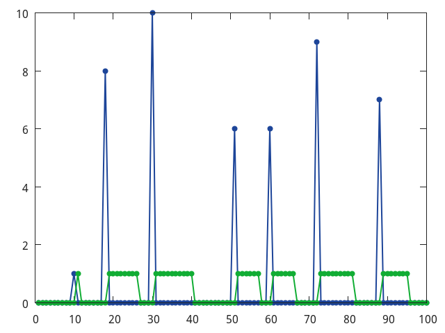
     • 输入：000050000000006000000这样100个数字
     • 输出：000001111100000111111这样100个数字
     • 每当输入出现impulse，如5时，输出延迟了1然后输出5个1，要rnn去学习这样的序列
     • rnn定义为hidden_size为20的简单rnn
   • 参考：深度学习笔记（五）用Torch实现RNN来制作一个神经网络计时器

   • 生成数据

     • 准备

     require 'torch'
     require 'gnuplot'
     math.randomseed(1) --[[种子，同一种子产生的随机数序列是相同，的，因此可以使用math.randomseed(os.time())避免随机数重合，参考http://blog.csdn.net/zhangxaochen/article/details/8095007]]
     sample_length = 100
     sample_amount = 10000
     X = torch.zeros(sample_length)
     Y = torch.zeros(sample_length)

     • 生成

       for n=2,sample_amount do
           sample_count = 0
           input = {}--[[Lua中数组，使用[]选择]]
           output = {}
            while sample_count < sample_length do
               t_blank = math.random(1,10)--[[产生1~10之间随机数]]
               t_intense = math.random(1,10)
               for i = 1,t_blank do
                 table插入(input, 0)
                 --[[table插入(table, pos, value), table.insert()函数在table的数组部分指定位置(pos)插入值为value的一个元素. pos参数可选, 默认为数组部分末尾, 参考http://www.cnblogs.com/whiteyun/archive/2009/08/10/1543139.html.]]
                 table插入(output, 0)
               end
                table插入(input, t_intense)
                table插入(output, 0)
               for i = 1,t_intense do
                table插入(input, 0)
                table插入(output, 1)
               end
               sample_count = sample_count+t_blank+t_intense+1
             end
         input = torch.Tensor(input)
         input = input[{{1, sample_length}}]--从input中取得1～sample_length的长度
         output = torch.Tensor(output)
         output = output[{{1, sample_length}}]
         X = X:cat(input,2)--将X和input连接起来，2是第2维度上连接
         --[[从input中取得1～sample_length的长度，
           如print(torch.cat(torch.ones(3,2),torch.zeros(2,2),1))会输出 
            1  1
            1  1
            1  1
            0  0
            0  0
           X=torch.cat(torch.ones(3),torch.zeros(3),2)会输出
           1  0
           1  0
           1  0
           ]]
         Y = Y:cat(output,2)
       end

     • 画图

       torch.save('data.t7', {X:t(), Y:t()}) --t()是取转置
       gnuplot.pngfigure('/media/majing/work/rnn/examples/torch-practice/rnn-timer/img/timer.png')
       gnuplot.plot({input},{output})
       gnuplot.plotflush()

     取一个X和Y的序列，如图
     

   • Minibatch

     local MinibatchLoader = {}
     MinibatchLoader.__index = MinibatchLoader
     function MinibatchLoader.create(batch_size)
     -- split_fractions is e.g. {0.9, 0.05, 0.05}
     
     local self = {}
     setmetatable(self, MinibatchLoader)
     --[[
         --定义2个表
             a = {5, 6}
             b = {7, 8}
         --用c来做Metatable
             c = {}
         --重定义加法操作
             c.__add = function(op1, op2)
                for _, item in ipairs(op2) do
                   table.insert(op1, item)
                end
                return op1
             end
         --将a的Metatable设置为c
             setmetatable(a, c)
         --d现在的样子是{5,6,7,8}
             d = a + b
             重定义了2个表的加法操作. 这个例子中将c的__add域改写后将a的Metatable设置为c, 当执行到加法的操作时, Lua首先会检查a是否有Metatable并且Metatable中是否存在__add域, 如果有则调用, 否则将检查b的条件(和a相同), 如果都没有则调用默认加法运算, 而table没有定义默认加法运算, 则会报错.参考http://www.cnblogs.com/simonw/archive/2007/01/17/622032.html
     ]]
     
     self.batch_size = batch_size
     self.batch_idx = 1
     
     local data_filename = 'data.t7'
     
     print('loading data files...')
     self.data = torch.load(data_filename)
     
     self.sample_size = self.data[1]:size(1)
     
     print(string.format('data load done.'))
     collectgarbage()
     return self
     end
     function MinibatchLoader:next_batch()
     
         X = self.data[1]:sub((self.batch_idx-1)*self.batch_size+1, self.batch_idx*self.batch_size)--origin, a batch data
         Y = self.data[2]:sub((self.batch_idx-1)*self.batch_size+1, self.batch_idx*self.batch_size)--target, a batch data
         self.batch_idx = self.batch_idx + 1--next batch
     
         if(self.batch_idx*self.batch_size > self.sample_size) then
             self.batch_idx = 1
         end
     
         table_x = {}
         table_y = {}
     
         for i=1,X:size(2) do
           table插入(table_x, X[{{},{i}}])
           table插入(table_y, Y[{{},{i}}])
         end
     
         return table_x, table_y
     end
     
     return MinibatchLoader

   • train

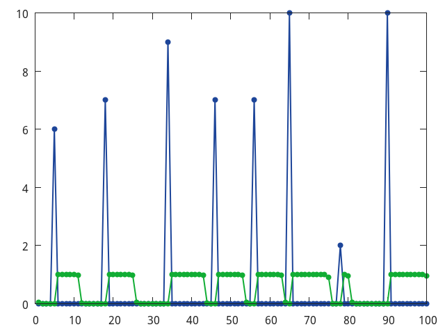
     require 'rnn'
     require 'gnuplot'
     
     batchSize = 8
     rho = 100
     hiddenSize = 20
     
     -- RNN
     
     batchLoader = require 'MinibatchLoader'
     loader = batchLoader.create(batchSize)
     
     r = nn.Recurrent(
        hiddenSize, nn.Linear(1, hiddenSize), 
        nn.Linear(hiddenSize, hiddenSize), nn.Sigmoid(), 
        rho
     )
     --[[
     隐藏层r的类型是nn.Recurrent。后面跟的参数依次分别是：
     1. 本层中包含的节点个数，为hiddenSize
     2. 前一层（也就是输入层）到本层的连接。这里是一个输入为1，输出为hiddenSize的线性连接。
     3. 本层节点到自身的反馈连接。这里是一个输入为hiddenSize，输出也是hiddenSize的线性连接。
     4. 本层输入和反馈连接所用的激活函数。这里用的是Sigmoid。
     5. Back propagation through time所进行的最大的次数。这里是rho = 100
     ]]
     
     
     rnn = nn.Sequential()
     rnn:add(nn.Sequencer(r))
     rnn:add(nn.Sequencer(nn.Linear(hiddenSize, 1)))
     rnn:add(nn.Sequencer(nn.Sigmoid()))
     --[[ 
     首先定义一个容器，然后添加刚才定义好的隐藏层r。随后添加隐藏层到输出层的连接，在这里用的是输入为20，输出为1的线性连接。最后接上一层Sigmoid函数。
     这里在定义网络的时候，每个具体的模块都是用nn.Sequencer的括号给括起来的。nn.Sequencer是一个修饰模块。所有经过nn.Sequencer包装过的模块都变得可以接受序列的输入。
     举个例子来说，假设有一个模块本来能够接受一个2维的Tensor作为输入，并输出另一个2维的Tensor。如果我们想把一系列的2维Tensor依次输入给这个模块，需要写一个for循环来实现。有了nn.Sequencer的修饰就不用这么麻烦了。只需要把这一系列的2维Tensor统一放到一个大的table里，然后一次性的丢给nn.Sequencer就行了。nn.Sequencer会把table中的Tensor依次放入网络，并将网络输出的Tensor也依次放入一个大的table中返回给你。
     ]]       
     
     
     criterion = nn.SequencerCriterion(nn.MSECriterion())
     --[[定义好了网络，接下来是定义评判标准]]
     
     lr = 0.01
     i = 1
     --[[
     接下来的事情又是例行公事了。向前传播，向后传播，更新参数.
     使用了MinibatchLoader（同目录下的MinibatchLoader.lua文件）来从data.t7中读取数据，每次读取8个序列，每个序列的时间长度是100。那么代码中inputs的类型是table，这个table中有100个元素，每个元素是一个2维8列1行的Tensor。在训练的时候，mini batch中8个序列中的每一个的第一个数据一起进入网络，接下来是8个排在第二的数据一起输入，如此迭代。
     ]]
     for n=1,6000 do
        -- prepare inputs and targets
        local inputs, targets = loader:next_batch()
     
        local outputs = rnn:forward(inputs)
        local err = criterion:forward(outputs, targets)
        print(i, err/rho)
        i = i + 1
        local gradOutputs = criterion:backward(outputs, targets)
        rnn:backward(inputs, gradOutputs)
        rnn:updateParameters(lr)
        rnn:zeroGradParameters()
     end
     
     --[[
     当训练完成之后，用其中的组输入放进网络观察其输出]]
     inputs, targets = loader:next_batch()
     outputs = rnn:forward(inputs)
     
     x={}
     y={}
     for i=1,100 do
        table插入(x,inputs[i][{1,1}])
        table插入(y,outputs[i][{1,1}])
     end
     
     x = torch.Tensor(x)
     y = torch.Tensor(y)
     
     gnuplot.pngfigure('timer.png')
     gnuplot.plot({x},{y})
     gnuplot.plotflush()
     

     结果显示入图

3. char-rnn

4. 4.