


http://blog.csdn.net/acdreamers/article/details/44663305
在上一篇文章中,讲述了广义线性模型。通过详细的讲解,针对某类指数分布族建立对应的广义线性模型。在本篇文章
中,将继续来探讨广义线性模型的一个重要例子,它可以看成是Logistic回归的扩展,即softmax回归。
我们知道Logistic回归只能进行二分类,因为它的随机变量的取值只能是0或者1,那么如果我们面对多分类问题怎么
办?比如要将一封新收到的邮件分为垃圾邮件,个人邮件,还是工作邮件;根据病人的病情预测病人属于哪种病;对于
诸如MNIST手写数字分类(MNIST是一个手写数字识别库,相见:http://yann.lecun.com/exdb/mnist/)。诸
如此类问题都涉及到多分类,那么今天要讲的softmax回归能解决这类问题。
在Logistic回归中,样本数据的值 ,而在softmax回归中
 ,其中
,其中 是类别种数,
比如在手写识别中 ,表示要识别的10个数字。设

那么

而且有

为了将多项式模型表述成指数分布族,先引入 ,它是一个
,它是一个 维的向量,那么

应用于一般线性模型, 必然是属于
必然是属于 个类中的一种。用
 表示
表示 为真,同样当
 为假时,有
为假时,有
 ,那么进一步得到联合分布的概率密度函数为

对比一下,可以得到

由于

那么最终得到

可以得到期望值为

接下来得到对数似然函数函数为

其中 是一个
是一个 的矩阵,代表这
 个类的所有训练参数,每个类的参数是一个
 维的向量。所以在
softmax回归中将 分类为类别
分类为类别 的概率为
的概率为

【tbw注:这里的p的写法,和Ng公开课里的写法并不一样,Ng里面因为无法求出第k个(用的是1减去前k-1个),因此最后得出的结果是1+j从1到k-1的加和】总之,不能用(k-1)加和来算p就是了,否则,Pk的概率永远为0
跟Logistic回归一样,softmax也可以用梯度下降法或者牛顿迭代法求解,对对数似然函数求偏导数,得到

然后我们可以通过梯度上升法来更新参数

注意这里 是第
是第 个类的所有参数,它是一个向量。
在softmax回归中直接用上述对数似然函数是不能更新参数的,因为它存在冗余的参数,通常用牛顿方法中的Hessian
矩阵也不可逆,是一个非凸函数,那么可以通过添加一个权重衰减项来修改代价函数,使得代价函数是凸函数,并且
得到的Hessian矩阵可逆。更多详情参考如下链接。
链接:http://deeplearning.stanford.edu/wiki/index.php/Softmax%E5%9B%9E%E5%BD%92
这里面也讲述了K个二元分类器与softmax的区别,值得学习。
Softmax回归
Contents[hide] |
简介
在本节中,我们介绍Softmax回归模型,该模型是logistic回归模型在多分类问题上的推广,在多分类问题中,类标签  可以取两个以上的值。 Softmax回归模型对于诸如MNIST手写数字分类等问题是很有用的,该问题的目的是辨识10个不同的单个数字。Softmax回归是有监督的,不过后面也会介绍它与深度学习/无监督学习方法的结合。(译者注: MNIST 是一个手写数字识别库,由NYU 的Yann LeCun 等人维护。http://yann.lecun.com/exdb/mnist/ )
回想一下在 logistic 回归中,我们的训练集由  个已标记的样本构成:
 ,其中输入特征
 。(我们对符号的约定如下:特征向量
  的维度为
的维度为  ,其中
,其中  对应截距项 。) 由于 logistic 回归是针对二分类问题的,因此类标记
  。假设函数(hypothesis function) 如下:

我们将训练模型参数  ,使其能够最小化代价函数 :
![\begin{align}J(\theta) = -\frac{1}{m} \left[ \sum_{i=1}^m y^{(i)} \log h_\theta(x^{(i)}) + (1-y^{(i)}) \log (1-h_\theta(x^{(i)})) \right]\end{align}](https://i-blog.csdnimg.cn/blog_migrate/50108045f56cfd2be293fd36791302aa.png)
在 softmax回归中,我们解决的是多分类问题(相对于 logistic 回归解决的二分类问题),类标 可以取  个不同的值(而不是 2 个)。因此,对于训练集 ,我们有
  。(注意此处的类别下标从 1 开始,而不是 0)。例如,在 MNIST 数字识别任务中,我们有
  个不同的类别。
对于给定的测试输入 ,我们想用假设函数针对每一个类别j估算出概率值  。也就是说,我们想估计 的每一种分类结果出现的概率。因此,我们的假设函数将要输出一个 维的向量(向量元素的和为1)来表示这 个估计的概率值。 具体地说,我们的假设函数
  形式如下:
形式如下:

其中  是模型的参数。请注意
  这一项对概率分布进行归一化,使得所有概率之和为 1 。
为了方便起见,我们同样使用符号 来表示全部的模型参数。在实现Softmax回归时,将 用一个  的矩阵来表示会很方便,该矩阵是将
  按行罗列起来得到的,如下所示:

代价函数
现在我们来介绍 softmax 回归算法的代价函数。在下面的公式中, 是示性函数,其取值规则为:
值为真的表达式

, 值为假的表达式  。举例来说,表达式
  的值为1 ,
 的值为 0。我们的代价函数为:
![\begin{align}J(\theta) = - \frac{1}{m} \left[ \sum_{i=1}^{m} \sum_{j=1}^{k} 1\left\{y^{(i)} = j\right\} \log \frac{e^{\theta_j^T x^{(i)}}}{\sum_{l=1}^k e^{ \theta_l^T x^{(i)} }}\right]\end{align}](https://i-blog.csdnimg.cn/blog_migrate/a073892ce762fc79f27dd3c5ed17c311.png)
值得注意的是,上述公式是logistic回归代价函数的推广。logistic回归代价函数可以改为:
![\begin{align}J(\theta) &= -\frac{1}{m} \left[ \sum_{i=1}^m (1-y^{(i)}) \log (1-h_\theta(x^{(i)})) + y^{(i)} \log h_\theta(x^{(i)}) \right] \\&= - \frac{1}{m} \left[ \sum_{i=1}^{m} \sum_{j=0}^{1} 1\left\{y^{(i)} = j\right\} \log p(y^{(i)} = j | x^{(i)} ; \theta) \right]\end{align}](https://i-blog.csdnimg.cn/blog_migrate/b3a78c38e828676839d41fffe51dfb27.png)
可以看到,Softmax代价函数与logistic 代价函数在形式上非常类似,只是在Softmax损失函数中对类标记的 个可能值进行了累加。注意在Softmax回归中将 分类为类别  的概率为:
的概率为:
-
 .
.
对于  的最小化问题,目前还没有闭式解法。因此,我们使用迭代的优化算法(例如梯度下降法,或 L-BFGS)。经过求导,我们得到梯度公式如下:
![\begin{align}\nabla_{\theta_j} J(\theta) = - \frac{1}{m} \sum_{i=1}^{m}{ \left[ x^{(i)} \left( 1\{ y^{(i)} = j\} - p(y^{(i)} = j | x^{(i)}; \theta) \right) \right] }\end{align}](https://i-blog.csdnimg.cn/blog_migrate/54cf0e3342849a42d2f6c5a5a6e17c05.png)
让我们来回顾一下符号 " " 的含义。
 本身是一个向量,它的第
  个元素
个元素  是 对
是 对 的第 个分量的偏导数。
有了上面的偏导数公式以后,我们就可以将它代入到梯度下降法等算法中,来最小化 。 例如,在梯度下降法的标准实现中,每一次迭代需要进行如下更新:  (
( )。
)。
当实现 softmax 回归算法时, 我们通常会使用上述代价函数的一个改进版本。具体来说,就是和权重衰减(weight decay)一起使用。我们接下来介绍使用它的动机和细节。
Softmax回归模型参数化的特点
Softmax 回归有一个不寻常的特点:它有一个“冗余”的参数集。为了便于阐述这一特点,假设我们从参数向量 中减去了向量  ,这时,每一个 都变成了
  ()。此时假设函数变成了以下的式子:

换句话说,从 中减去 完全不影响假设函数的预测结果!这表明前面的 softmax 回归模型中存在冗余的参数。更正式一点来说, Softmax 模型被过度参数化了。对于任意一个用于拟合数据的假设函数,可以求出多组参数值,这些参数得到的是完全相同的假设函数  。
。
进一步而言,如果参数  是代价函数 的极小值点,那么
  同样也是它的极小值点,其中 可以为任意向量。因此使 最小化的解不是唯一的。(有趣的是,由于 仍然是一个凸函数,因此梯度下降时不会遇到局部最优解的问题。但是 Hessian 矩阵是奇异的/不可逆的,这会直接导致采用牛顿法优化就遇到数值计算的问题)
注意,当  时,我们总是可以将
  替换为
替换为 (即替换为全零向量),并且这种变换不会影响假设函数。因此我们可以去掉参数向量 (或者其他 中的任意一个)而不影响假设函数的表达能力。实际上,与其优化全部的 个参数 (其中
  ),我们可以令
  ,只优化剩余的
  个参数,这样算法依然能够正常工作。
在实际应用中,为了使算法实现更简单清楚,往往保留所有参数  ,而不任意地将某一参数设置为 0。但此时我们需要对代价函数做一个改动:加入权重衰减。权重衰减可以解决 softmax 回归的参数冗余所带来的数值问题。
权重衰减
我们通过添加一个权重衰减项  来修改代价函数,这个衰减项会惩罚过大的参数值,现在我们的代价函数变为:
![\begin{align}J(\theta) = - \frac{1}{m} \left[ \sum_{i=1}^{m} \sum_{j=1}^{k} 1\left\{y^{(i)} = j\right\} \log \frac{e^{\theta_j^T x^{(i)}}}{\sum_{l=1}^k e^{ \theta_l^T x^{(i)} }} \right] + \frac{\lambda}{2} \sum_{i=1}^k \sum_{j=0}^n \theta_{ij}^2\end{align}](https://i-blog.csdnimg.cn/blog_migrate/bc700706ad83bdf7e6b610573463ffb1.png)
有了这个权重衰减项以后 ( ),代价函数就变成了严格的凸函数,这样就可以保证得到唯一的解了。 此时的 Hessian矩阵变为可逆矩阵,并且因为是凸函数,梯度下降法和 L-BFGS 等算法可以保证收敛到全局最优解。
为了使用优化算法,我们需要求得这个新函数 的导数,如下:
![\begin{align}\nabla_{\theta_j} J(\theta) = - \frac{1}{m} \sum_{i=1}^{m}{ \left[ x^{(i)} ( 1\{ y^{(i)} = j\} - p(y^{(i)} = j | x^{(i)}; \theta) ) \right] } + \lambda \theta_j\end{align}](https://i-blog.csdnimg.cn/blog_migrate/1e2bd9b5ae929e485dc03f413d9e163f.png)
通过最小化 ,我们就能实现一个可用的 softmax 回归模型。
Softmax回归与Logistic 回归的关系
当类别数  时,softmax 回归退化为 logistic 回归。这表明 softmax 回归是 logistic 回归的一般形式。具体地说,当 时,softmax 回归的假设函数为:

利用softmax回归参数冗余的特点,我们令 ,并且从两个参数向量中都减去向量 ,得到:

因此,用  来表示
来表示 ,我们就会发现 softmax 回归器预测其中一个类别的概率为
  ,另一个类别概率的为
  ,这与 logistic回归是一致的。
Softmax 回归 vs. k 个二元分类器
如果你在开发一个音乐分类的应用,需要对k种类型的音乐进行识别,那么是选择使用 softmax 分类器呢,还是使用 logistic 回归算法建立 k 个独立的二元分类器呢?
这一选择取决于你的类别之间是否互斥,例如,如果你有四个类别的音乐,分别为:古典音乐、乡村音乐、摇滚乐和爵士乐,那么你可以假设每个训练样本只会被打上一个标签(即:一首歌只能属于这四种音乐类型的其中一种),此时你应该使用类别数 k = 4 的softmax回归。(如果在你的数据集中,有的歌曲不属于以上四类的其中任何一类,那么你可以添加一个“其他类”,并将类别数 k 设为5。)
如果你的四个类别如下:人声音乐、舞曲、影视原声、流行歌曲,那么这些类别之间并不是互斥的。例如:一首歌曲可以来源于影视原声,同时也包含人声 。这种情况下,使用4个二分类的 logistic 回归分类器更为合适。这样,对于每个新的音乐作品 ,我们的算法可以分别判断它是否属于各个类别。
现在我们来看一个计算视觉领域的例子,你的任务是将图像分到三个不同类别中。(i) 假设这三个类别分别是:室内场景、户外城区场景、户外荒野场景。你会使用sofmax回归还是 3个logistic 回归分类器呢? (ii) 现在假设这三个类别分别是室内场景、黑白图片、包含人物的图片,你又会选择 softmax 回归还是多个 logistic 回归分类器呢?
在第一个例子中,三个类别是互斥的,因此更适于选择softmax回归分类器 。而在第二个例子中,建立三个独立的 logistic回归分类器更加合适。
中英文对照
- Softmax回归 Softmax Regression
- 有监督学习 supervised learning
- 无监督学习 unsupervised learning
- 深度学习 deep learning
- logistic回归 logistic regression
- 截距项 intercept term
- 二元分类 binary classification
- 类型标记 class labels
- 估值函数/估计值 hypothesis
- 代价函数 cost function
- 多元分类 multi-class classification
- 权重衰减 weight decay
中文译者
曾俊瑀(knighterzjy@gmail.com), 王方(fangkey@gmail.com),王文中(wangwenzhong@ymail.com)
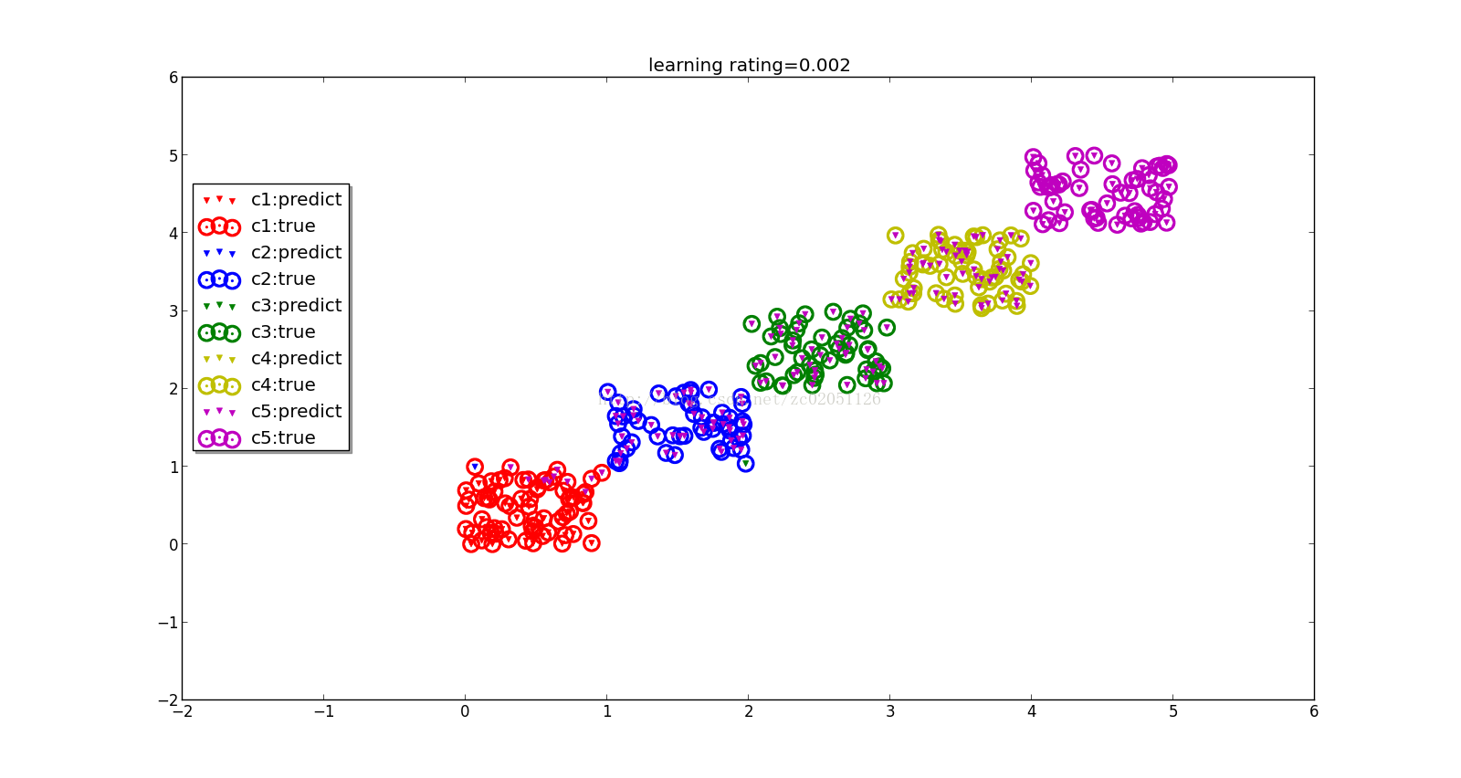
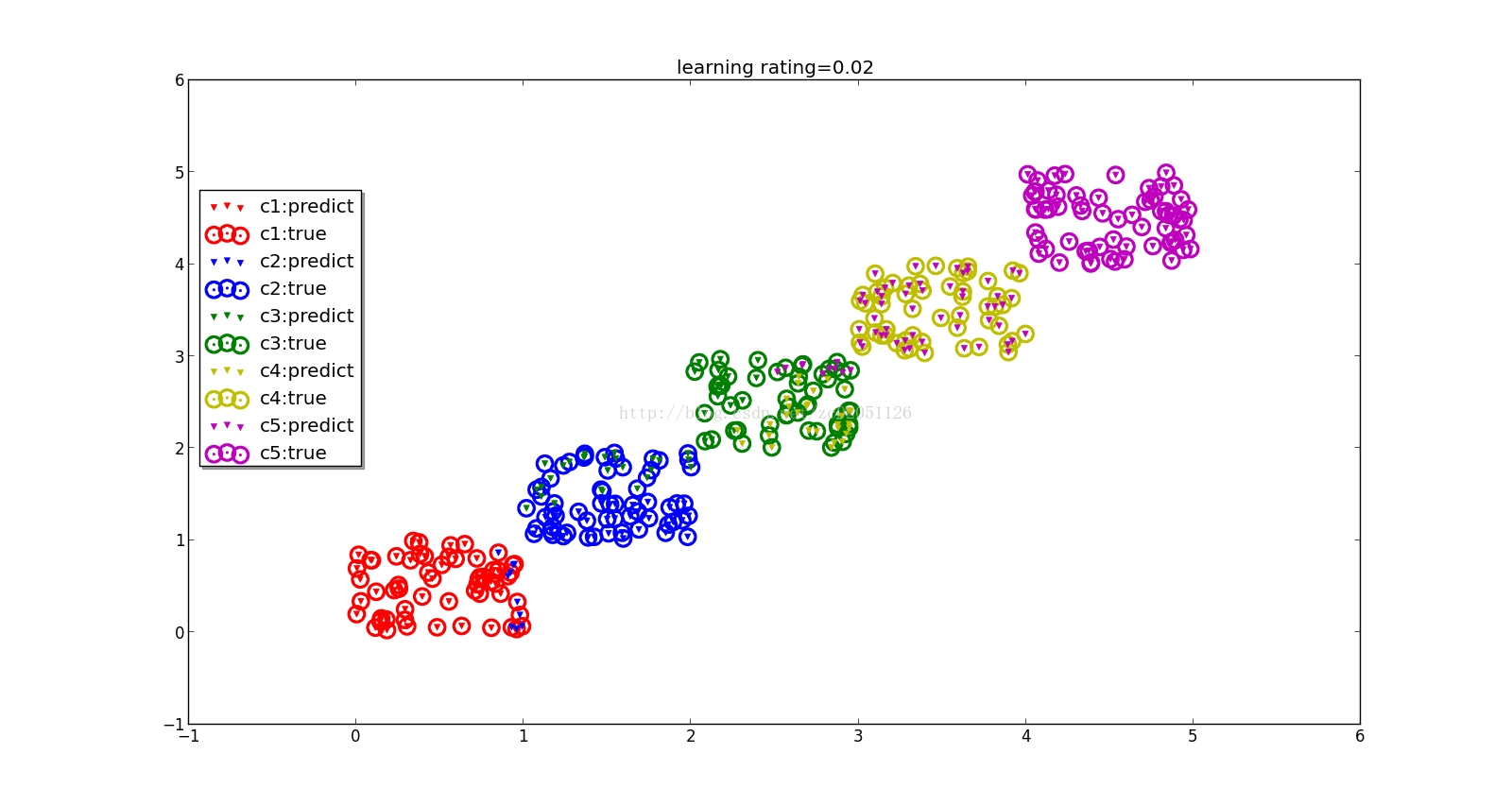
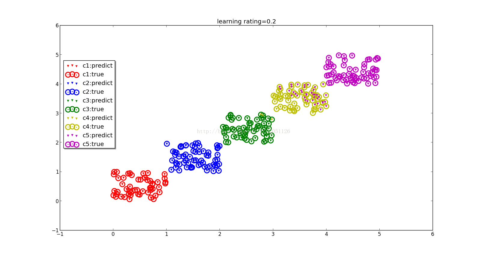
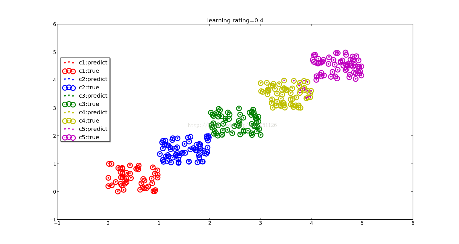
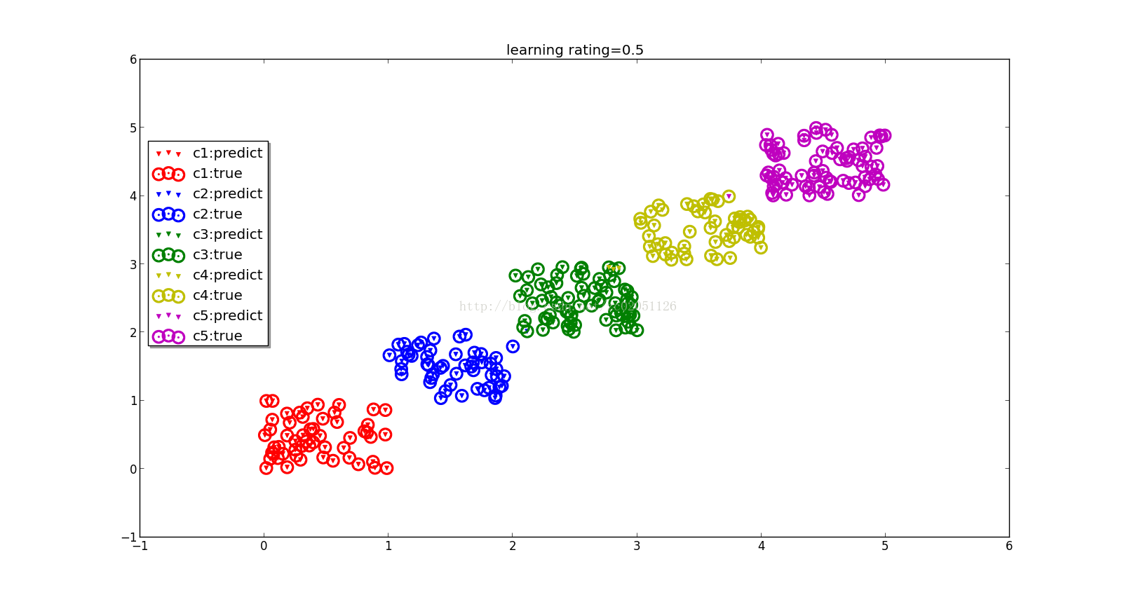
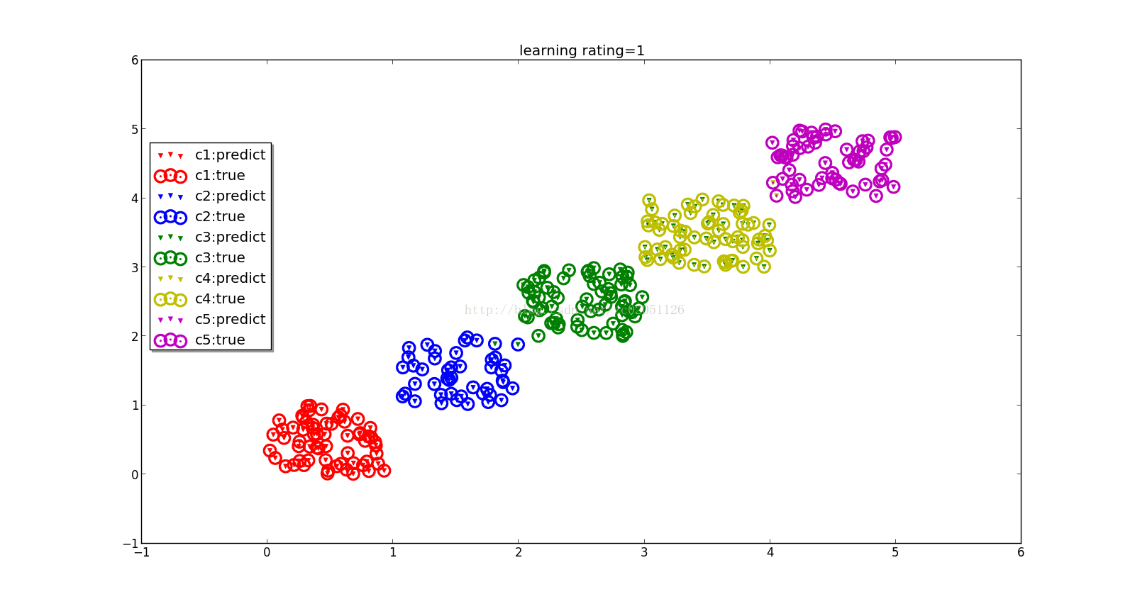
终于实现了逻辑回归的扩展版本,训练方法采用梯度下降法,这种方法对学习率的要求比较高,不同的学习率可能导致结果大相径庭。见相关图
参考资料:http://deeplearning.stanford.edu/wiki/index.php/Softmax%E5%9B%9E%E5%BD%92
Python代码如下:
- import numpy as np
- import matplotlib.pylab as plt
- import copy
- from scipy.linalg import norm
- from math import pow
- from scipy.optimize import fminbound,minimize
- import random
- def _dot(a, b):
- mat_dot = np.dot(a, b)
- return np.exp(mat_dot)
- def condProb(theta, thetai, xi):
- numerator = _dot(thetai, xi.transpose())
- denominator = _dot(theta, xi.transpose())
- denominator = np.sum(denominator, axis=0)
- p = numerator / denominator
- return p
- def costFunc(alfa, *args):
- i = args[2]
- original_thetai = args[0]
- delta_thetai = args[1]
- x = args[3]
- y = args[4]
- lamta = args[5]
- labels = set(y)
- thetai = original_thetai
- thetai[i, :] = thetai[i, :] - alfa * delta_thetai
- k = 0
- sum_log_p = 0.0
- for label in labels:
- index = y == label
- xi = x[index]
- p = condProb(original_thetai,thetai[k, :], xi)
- log_p = np.log10(p)
- sum_log_p = sum_log_p + log_p.sum()
- k = k + 1
- r = -sum_log_p / x.shape[0]+ (lamta / 2.0) * pow(norm(thetai),2)
- #print r ,alfa
- return r
- class Softmax:
- def __init__(self, alfa, lamda, feature_num, label_mum, run_times = 500, col = 1e-6):
- self.alfa = alfa
- self.lamda = lamda
- self.feature_num = feature_num
- self.label_num = label_mum
- self.run_times = run_times
- self.col = col
- self.theta = np.random.random((label_mum, feature_num + 1))+1.0
- def oneDimSearch(self, original_thetai,delta_thetai,i,x,y ,lamta):
- res = minimize(costFunc, 0.0, method = 'Powell', args =(original_thetai,delta_thetai,i,x,y ,lamta))
- return res.x
- def train(self, x, y):
- tmp = np.ones((x.shape[0], x.shape[1] + 1))
- tmp[:,1:tmp.shape[1]] = x
- x = tmp
- del tmp
- labels = set(y)
- self.errors = []
- old_alfa = self.alfa
- for kk in range(0, self.run_times):
- i = 0
- for label in labels:
- tmp_theta = copy.deepcopy(self.theta)
- one = np.zeros(x.shape[0])
- index = y == label
- one[index] = 1.0
- thetai = np.array([self.theta[i, :]])
- prob = self.condProb(thetai, x)
- prob = np.array([one - prob])
- prob = prob.transpose()
- delta_thetai = - np.sum(x * prob, axis = 0)/ x.shape[0] + self.lamda * self.theta[i, :]
- #alfa = self.oneDimSearch(self.theta,delta_thetai,i,x,y ,self.lamda)#一维搜索法寻找最优的学习率,没有实现
- self.theta[i,:] = self.theta[i,:] - self.alfa * np.array([delta_thetai])
- i = i + 1
- self.errors.append(self.performance(tmp_theta))
- def performance(self, tmp_theta):
- return norm(self.theta - tmp_theta)
- def dot(self, a, b):
- mat_dot = np.dot(a, b)
- return np.exp(mat_dot)
- def condProb(self, thetai, xi):
- numerator = self.dot(thetai, xi.transpose())
- denominator = self.dot(self.theta, xi.transpose())
- denominator = np.sum(denominator, axis=0)
- p = numerator[0] / denominator
- return p
- def predict(self, x):
- tmp = np.ones((x.shape[0], x.shape[1] + 1))
- tmp[:,1:tmp.shape[1]] = x
- x = tmp
- row = x.shape[0]
- col = self.theta.shape[0]
- pre_res = np.zeros((row, col))
- for i in range(0, row):
- xi = x[i, :]
- for j in range(0, col):
- thetai = self.theta[j, :]
- p = self.condProb(np.array([thetai]), np.array([xi]))
- pre_res[i, j] = p
- r = []
- for i in range(0, row):
- tmp = []
- line = pre_res[i, :]
- ind = line.argmax()
- tmp.append(ind)
- tmp.append(line[ind])
- r.append(tmp)
- return np.array(r)
- def evaluate(self):
- pass
- def samples(sample_num, feature_num, label_num):
- n = int(sample_num / label_num)
- x = np.zeros((n*label_num, feature_num))
- y = np.zeros(n*label_num, dtype=np.int)
- for i in range(0, label_num):
- x[i*n : i*n + n, :] = np.random.random((n, feature_num)) + i
- y[i*n : i*n + n] = i
- return [x, y]
- def save(name, x, y):
- writer = open(name, 'w')
- for i in range(0, x.shape[0]):
- for j in range(0, x.shape[1]):
- writer.write(str(x[i,j]) + ' ')
- writer.write(str(y[i])+ '\n')
- writer.close()
- def load(name):
- x = []
- y = []
- for line in open(name, 'r'):
- ele = line.split(' ')
- tmp = []
- for i in range(0, len(ele) - 1):
- tmp.append(float(ele[i]))
- x.append(tmp)
- y.append(int(ele[len(ele) - 1]))
- return [x, y]
- def plotRes(pre, real, test_x,l):
- s = set(pre)
- col = ['r','b','g','y','m']
- fig = plt.figure()
- ax = fig.add_subplot(111)
- for i in range(0, len(s)):
- index1 = pre == i
- index2 = real == i
- x1 = test_x[index1, :]
- x2 = test_x[index2, :]
- ax.scatter(x1[:,0],x1[:,1],color=col[i],marker='v',linewidths=0.5)
- ax.scatter(x2[:,0],x2[:,1],color=col[i],marker='.',linewidths=12)
- plt.title('learning rating='+str(l))
- plt.legend(('c1:predict','c1:true',\
- 'c2:predict','c2:true',
- 'c3:predict','c3:true',
- 'c4:predict','c4:true',
- 'c5:predict','c5:true'), shadow = True, loc = (0.01, 0.4))
- plt.show()
- if __name__ == '__main__':
- #[x, y] = samples(1000, 2, 5)
- #save('data.txt', x, y)
- [x, y] = load('data.txt')
- index= range(0, len(x))
- random.shuffle(index)
- x = np.array(x)
- y = np.array(y)
- x_train = x[index[0:700],:]
- y_train = y[index[0:700]]
- softmax = Softmax(0.4, 0.0, 2, 5)#这里讲第二个参数设置为0.0,即不用正则化,因为模型中没有高次项,用正则化反而使效果变差
- softmax.train(x_train, y_train)
- x_test = x[index[700:1000],:]
- y_test = y[index[700:1000]]
- r= softmax.predict(x_test)
- plotRes(r[:,0],y_test,x_test,softmax.alfa)
- t = r[:,0] != y_test
- o = np.zeros(len(t))
- o[t] = 1
- err = sum(o)


 114
114

 被折叠的 条评论
为什么被折叠?
被折叠的 条评论
为什么被折叠?
 到【灌水乐园】发言


