Paper Reading — Vision Transformer / Swin Transformer

最新推荐文章于 2024-07-25 22:26:10 发布

自动驾驶之星

最新推荐文章于 2024-07-25 22:26:10 发布

阅读量955

点赞数 10

分类专栏： Paper Reading 自动驾驶文章标签： transformer 深度学习人工智能自动驾驶

本文链接：https://blog.csdn.net/tjy792864625/article/details/138860408

版权

Paper Reading 同时被 2 个专栏收录

4 篇文章 0 订阅

订阅专栏

自动驾驶

1 篇文章 0 订阅

订阅专栏

Vision Transformer

发表单位：Google
发表时间：2020年

1. inductive bias的理解

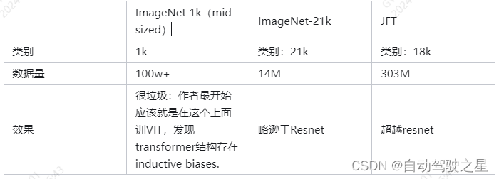
VIT验证了一个重要的结论：当训练数据达到千万级别的时候，transformer结构可以跨过本身缺少的inductive bias，达到比传统的resnet更好的效果。
When trained on mid-sized datasets such as ImageNet without strong regularization, these models yield modest accuracies of a few percentage points below ResNets of comparable size. This seemingly discouraging outcome may be expected: Transformers lack some of the inductive biases.
However, the picture changes if the models are trained on larger datasets (14M-300M images). We find that large scale training trumps inductive bias. Our Vision Transformer (ViT) attains excellent results when pre-trained at sufficient scale and transferred to tasks with fewer datapoints. When pre-trained on the public ImageNet-21k dataset or the in-house JFT-300M dataset, ViT approaches or beats state of the art on multiple image recognition benchmarks.
“归纳偏置”（inductive bias）是指模型在学习时对数据的某些先验假设或偏好。
对于图像数据来说，归纳偏置体现在：
空间局部性：图像在空间上相邻的位置往往具有相关性。因此，CNN通过卷积可以获取到图像中的局部特征。
平移不变性：图像中的目标物体在图像中移动，它依然还是该物体。CNN通过卷积和池化等操作，神经网络能够实现对于物体在图像中位置的不敏感性。
尺度不变性：图像中的目标物体的大小发生变化，它依然还是该物体。CNN通过池化层等操作，可以在一定程度上对尺度变化具有不变性。
换句话说，CNN的结构的设计是适应于图像的这三个先验信息的。但是transformer的结构设计最开始是适应于文本数据的，文本数据的归纳偏置与图像不同，它体现在：
自注意力机制：需要通过self-attention关注到序列中所有位置的信息（而不仅仅是局部的上下文，像图像数据那样），因为我们说话时的某个字，可能和整句话中的每个字都有关联。

2. 数据集

VIT的使用方法：在大数据集上进行pre-train，然后在任务对应的小数据集上进行finetune。一套组合拳下来，效果超越了Resnet。

3. VIT结构梳理：

3.1 整体结构图

VIT结构图
这是一段CLIP中VIT的代码，与原始的VIT略有不同：

def forward(self, x: torch.Tensor):
    x = self.conv1(x)  # shape = [*, width, grid, grid]
    x = x.reshape(x.shape[0], x.shape[1], -1)  # shape = [*, width, grid ** 2]
    x = x.permute(0, 2, 1)  # shape = [*, grid ** 2, width]
    # class embedding
    x = torch.cat([self.class_embedding.to(x.dtype) + torch.zeros(x.shape[0], 1, x.shape[-1], dtype=x.dtype, device=x.device), x], dim=1)  # shape = [*, grid ** 2 + 1, width]
    # pos embedding
    x = x + self.positional_embedding.to(x.dtype)
    #layer norm
    x = self.ln_pre(x)
    # transformer
    x = x.permute(1, 0, 2)  # NLD -> LND
    x = self.transformer(x)
    x = x.permute(1, 0, 2)  # LND -> NLD
    # layer norm
    x = self.ln_post(x[:, 0, :])

    # 线性映射
    if self.proj is not None:
        x = x @ self.proj
    return x

3.2 tensor 数据流

1. 输入数据的预处理
从debug信息可以看出，输入为224 * 224的图像。conv1是一个stride为32，kernel_size为32的，输入输出通道分别为3和768的卷积核。相当于是卷积核在每个3232的patch上提取特征，生成的是77个patch对应的768维特征。

2. Class embedding
从整体结构图中可以看出，VIT仿照Bert结构，在所有embeddings（这些embeddings在VIT中是从每个patch中提取的特征）的最前面加上了一个用于分类的可学习的class embedding。在self attention的过程中，这个class embedding可以浏览到所有图像embeddings中的内容。相当于是加权所有patch的特征，代表整张图像的特征，最后用于输出一个分类的结果。

self.class_embedding.shape
#debug info
#torch.Size([768])

x.shape
#debug info
#torch.Size([1,50,768])

3. Position embedding
图像分成7*7个patch 外加一个class embedding，一共是50个768维度的embeddings。因此，对应的可学习的position embedding也是50个。

self.positional_embeddig.shape

# debug info
# torch.Size([50,768])

这里需要思考下：预训练的时候是固定224224分辨率的图，在finetune下游分类任务的时候，通常是更大分辨率的图像。我们不必担心embeddings数量对于transformer网络结构本身的影响，因为QKV本身就是矩阵乘法，只要向量长度（hidden dim）不变就行，就可以在pretrain的transformer网络params的基础上继续finetune。但是embeddings数量的变化，会直接使得position embedding失去意义，比如77变成14*14，这个时候就需要用到插值的方法来初始化pretrain模型的position embedding参数，重新赋予它意义，然后进行finetune。
4. Transformer

class QuickGELU(nn.Module):
    def forward(self, x: torch.Tensor):
        return x * torch.sigmoid(1.702 * x)

class ResidualAttentionBlock(nn.Module):
    def __init__(self, d_model: int, n_head: int, attn_mask: torch.Tensor = None):
        super().__init__()

        self.attn = nn.MultiheadAttention(d_model, n_head)
        self.ln_1 = LayerNorm(d_model)
        self.mlp = nn.Sequential(OrderedDict([
            ("c_fc", nn.Linear(d_model, d_model * 4)),
            ("gelu", QuickGELU()),
            ("c_proj", nn.Linear(d_model * 4, d_model))
        ]))
        self.ln_2 = LayerNorm(d_model)
        self.attn_mask = attn_mask

    def attention(self, x: torch.Tensor):
        self.attn_mask = self.attn_mask.to(dtype=x.dtype, device=x.device) if self.attn_mask is not None else None
        return self.attn(x, x, x, need_weights=False, attn_mask=self.attn_mask)[0]

    def forward(self, x: torch.Tensor):
        x = x + self.attention(self.ln_1(x))
        x = x + self.mlp(self.ln_2(x))
        return x

class Transformer(nn.Module):
    def __init__(self, width: int, layers: int, heads: int, attn_mask: torch.Tensor = None):
        super().__init__()
        self.width = width
        self.layers = layers
        self.resblocks = nn.Sequential(*[ResidualAttentionBlock(width, heads, attn_mask) for _ in range(layers)])

    def forward(self, x: torch.Tensor):
        return self.resblocks(x)

没什么可说的，设置Layers层数，hidden dim，heads，MLP size就好了。
Config Table

5. 下游任务

# layer norm
x = self.ln_post(x[:,0,:])

#线性映射
if self.proj is not None:
	x = x @ self.proj
return x

只用class embedding（768维度的特征向量），进一步进行线性映射到新的特征空间。对于下游的分类任务，可以接一个FC层得到最终的分类结果。
在CLIP的工作中，class embedding被映射到另外一个512维的特征空间中，然后与文本提取的特征之间计算相似度。这个时候，所谓的class embedding所代表的就是整张图像的特征。

-------------------------------------------------------------------------------------------

Swin Transformer

原文：https://arxiv.org/abs/2103.14030
2021年微软研究院 ICCV Best Paper

背景

Google Brain团队在2020年提出了Vision Transformer（VIT），但是VIT存在的问题是它的结构依然是适用于文本任务的，也就是global attention。VIT原文中用了一定的篇幅强调了transformer结构用于视觉任务中需要大量的数据集来训练，原因就是所谓的 inductive biases。
大概意思就是文本任务和视觉任务的特点不同，像gpt这种文本预测的任务，每预测一个词，它需要把前面所有的词都看一遍，transformer中不管是self-attention还是cross-attention都是在特征的整个集合中进行的，这就是为啥transformer最开始就是用于NLP的。
而我们知道，图像特征的特点是Local的（不管是传统的surf、orb，还是CNN都是在局部提取特征），VIT沿用了transformer的原始设计，在全局计算attention，这样做不光不符合图像特征的特点，而且计算量也非常大。另外，VIT也没有尝试将多尺度加进去。因此在分割、检测任务上也一般，它只是提供了vision领域一种transformer最早的范式。

1. Swin Transformer的结构总览

Swin Transformer整体结构

1.1 Swin Transformer Blocks 以外其他的结构设计：

Patch Partition
将图像分块，每个patch大小为44，然后flatten程44*3 = 48维度，最后一个patch就代表一个48维度的token embedding。
Linear Embedding
将patch原始的48维像素值映射到某个特征空间中，特征维度为C
Patch Merging
这是一种降采样的方式，经过Patch Merging后整个feature map分辨率2倍降采样，且通道数*2（后面展开说）

1.2 Swin Transformer Blocks：

W-MSA(Window-Multi Self Attention)
每m*m个patch作为一个window，在这个window里面进行self-attention
SW-MSA(Shift Window-Multi Self Attention)
对Window的形状做一些微调，让W-MSA中设计的不同window之间也有一些信息融合（这块感觉有点像传统图像增强中一些基于分块的方法，在边界做一些融合过度）

1.3 Patch与Window：

patch：这个图中最小的方格（灰色方格）表示一个patch，一个patch也是一个token，也是一个像素点。比如最下边这层feature map上一个小方格patch就是由443的原图flatten成的48维向量，也就是最初始的token。
window：由灰色方格组成的红色方格表示一个window。
多尺度特征
从上图中可以看出，不同层的feature map上的一个patch/token 所对应原图上的图像块尺寸是不同的，这个思想就类似金字塔的多尺度。

2. Patch Partition

Patch Partition是将原图上一个个4×4×3通道的图像块展开拉平成48维向量的过程。

3. Patch Merging 结构

Patch Merging总体来讲是一个将4×4个patch转换成2×2×4个小的patch的过程。

Patch Merging示意图

具体就是把4*4个patch拆分并concat到一起。整体feature map的分辨率更小，同奥数更多。下图中一个方格表示一个像素。
拆分 + concat
然后分别经过Layer Norm层和另外一层linear：
特征压缩
OK，那么对一个完整的feature map上的所有patch都做Patching Merging的操作，最终的结果就是这个feature map的分辨率会2倍下采样，通道数会倍数乘2。

4. Swin Transformer Block

4.1 W-MSA(Window-Multi Self Attention)

用一句话解释就是在window中做self attention。以Swin Transformer的中间这一层处理为例，假设一个windows包含4×4个patch，那么W-MSA只在windows中做self attention。
Window-Multi Self Attention

4.2 SW-MSA（Shift Window-Multi Self Attention）

同样以中间这层feature map为例，对window的形状和size做微调，layerL+1层第一行的第二个windows中的tokens在做self attention的时候相当于是把layerL层的左上角和右上角windows中的token做了特征融合。
Shift Window-Multi self Attention

为了计算的方便，作者实际上由加了一些矩阵的循环移位和mask操作：
在这里插入图片描述

总结

Swin transformer 是对transformer的范式做了一些更适合视觉任务的优化。用window和shift-window的方法来让提取的图像特征在局部做一些attention，并在相邻的windows之间也做了特征融合的处理。在商汤的deformable detr中也用到了类似这种将local feature与transformer相结合的思想。
另外，Swin Transformer 可以在不同尺度上提取图像特征，对分割、检测任务更友好。
从现在这个时间节点来看，Swin Transformer已经在很多视觉任务中作为backbone来提取特征，例如：Dino，Grounding-Dino等等。

自动驾驶之星

关注

10
点赞
踩
19

收藏

觉得还不错? 一键收藏
1
评论
Paper Reading — Vision Transformer / Swin Transformer

这篇主要解析两篇文章：1. google在vision transformer领域的开山之作，首次将transformer结构用于视觉任务中。2. 微软推出的Swin transformer，2021年的ICCV Best Paper。Swin transformer结构已作为图像特征提取backbone，应用于Dino，Grounding-Dino（检测）以及多模融合等领域的工作中。
复制链接

扫一扫