人工智能学习-机器学习基本原理（二）

2 机器学习基本原理

2.1 基本数学知识

标量：标量也就是一个单独的数

向量：类似[1,2,3,4]被称之为向量，是一列数；其中可以进行的运算有加法运算以及向量之间做内积

​ 向量加法：i.e. [a1,a2,a3]+[b1,b2,b3]=[a1+b1,a2+b2,a3+b3]

​ 向量内积：i.e. [a1,a2,a3]*[b1,b2,b3]= a1*b1+a2*b2+a3*b3

张量：张量是Pytoch框架中通用的数据类型，类似矩阵之类的数据，都必须转换为张量才能输入Pytorch框架中以供模型进行训练

矩阵:矩阵是一组具有行列的数列，其中最重要的运算法则是矩阵乘法满足结合律以及分配律

​ 矩阵乘法：a=N*M, b=M*C 则a*b=N*C

​ 矩阵点乘：对位相乘，前提条件是两个矩阵的形状必须一致

导数：通俗的理解是导数是对应函数在某一点上的变化趋势
$$存在f(x),f^{\prime }(x)=\underset{h\to 0}{\lim }\frac{f(x+h)-f(x)}{f(x)}$$

2.2 模拟机器学习实现

概述：该代码主要是从最底层的方式去实现机器学习的过程，不会使用框架相关操作。

import sys
import math

# 1、自造标准输入输出
# X = [0.01*x for x in range(100)]
# Y = [2*i**2+3*i+4 for i in X]

X_true = [0.0, 0.01, 0.02, 0.03, 0.04, 0.05, 0.06, 0.07, 0.08, 0.09, 0.1, 0.11, 0.12, 0.13, 0.14, 0.15, 0.16, 0.17, 0.18, 0.19, 0.2, 0.21, 0.22, 0.23, 0.24, 0.25, 0.26, 0.27, 0.28, 0.29, 0.3, 0.31, 0.32, 0.33, 0.34, 0.35000000000000003, 0.36, 0.37, 0.38, 0.39, 0.4, 0.41000000000000003, 0.42, 0.43, 0.44, 0.45, 0.46, 0.47000000000000003, 0.48, 0.49, 0.5, 0.51, 0.52, 0.53, 0.54, 0.55, 0.56, 0.5700000000000001, 0.58, 0.59, 0.6, 0.61, 0.62, 0.63, 0.64, 0.65, 0.66, 0.67, 0.68, 0.6900000000000001, 0.7000000000000001, 0.71, 0.72, 0.73, 0.74, 0.75, 0.76, 0.77, 0.78, 0.79, 0.8, 0.81, 0.8200000000000001, 0.8300000000000001, 0.84, 0.85, 0.86, 0.87, 0.88, 0.89, 0.9, 0.91, 0.92, 0.93, 0.9400000000000001, 0.9500000000000001, 0.96, 0.97, 0.98, 0.99]
Y_true = [6.0, 6.0302, 6.0608, 6.0918, 6.1232, 6.155, 6.1872, 6.2198, 6.2528, 6.2862, 6.32, 6.3542, 6.3888, 6.4238, 6.4592, 6.495, 6.5312, 6.5678, 6.6048, 6.6422, 6.68, 6.7181999999999995, 6.7568, 6.7958, 6.8352, 6.875, 6.9152000000000005, 6.9558, 6.9968, 7.0382, 7.08, 7.122199999999999, 7.1648, 7.2078, 7.2512, 7.295, 7.3392, 7.3838, 7.4288, 7.4742, 7.5200000000000005, 7.5662, 7.6128, 7.6598, 7.7072, 7.755, 7.8032, 7.851800000000001, 7.9008, 7.9502, 8.0, 8.0502, 8.1008, 8.1518, 8.2032, 8.255, 8.3072, 8.3598, 8.4128, 8.4662, 8.52, 8.574200000000001, 8.6288, 8.6838, 8.7392, 8.795, 8.8512, 8.9078, 8.9648, 9.022200000000002, 9.08, 9.1382, 9.1968, 9.2558, 9.3152, 9.375, 9.4352, 9.4958, 9.556799999999999, 9.6182, 9.68, 9.7422, 9.8048, 9.8678, 9.9312, 9.995, 10.0592, 10.1238, 10.1888, 10.2542, 10.32, 10.3862, 10.4528, 10.5198, 10.587200000000001, 10.655000000000001, 10.7232, 10.7918, 10.8608, 10.9302]# 2、定义并随机初始化权重以及学习率
w1, w2, w3 = -1, 0, 1       # 权重
lr = 0.1         # 学习率


# 3、定义func、loss
def func(x):
    return w1*x**2+w2*x+w3


def loss(y_pred, y_true):
    loss = (y_pred-y_true) ** 2
    return loss


# 4、训练模型
for rounds in range(1000):
    loss_sum = 0
    loss_value = 0        # 损失值
    for x, y_standard in zip(X_true, Y_true):
        y_pred = func(x)
        loss_sum += loss(y_pred, y_standard)
        # 梯度计算
        grad_w1 = 2*(y_pred-y_standard)*x**2
        grad_w2 = 2*(y_pred-y_standard)*x
        grad_w3 = 2*(y_pred-y_standard)
        #权重更新
        w1 = w1-lr*grad_w1
        w2 = w2-lr*grad_w2
        w3 = w3-lr*grad_w3
    loss_value = loss_sum/100
    if loss_value< 0.001:
        break
# 5、输出权重
print("权重：w1=%f,w2=%f,w3=%f" % (w1, w2, w3))

最终结果：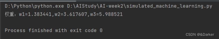

2.3 pytorch框架基本组件

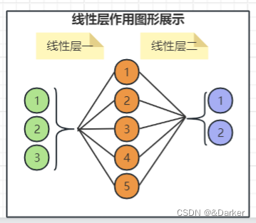
2.3.1 线性层

概述：线性层是其网络结构中最基本的一层，能够获取到训练数据的数据特征

基本形式：y=w*x+b,其中w,b为训练参数。

2.3.2 激活函数

概述：该函数的作用使的函数具有非线性的作用，例如一个分类任务中你无法通过一条直线将散乱的数据分为两类而必须通过一条曲线来进行数据的分类。

常用的激活函数：

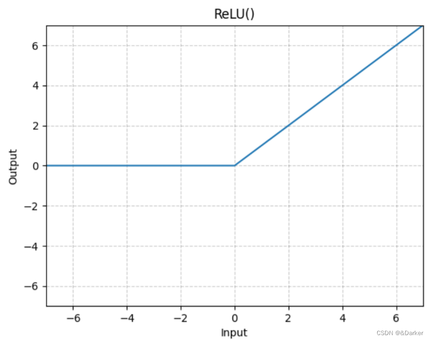
a.ReLU:
$$ReLU(x)=(x{)}^{+}=max(x,0)$$

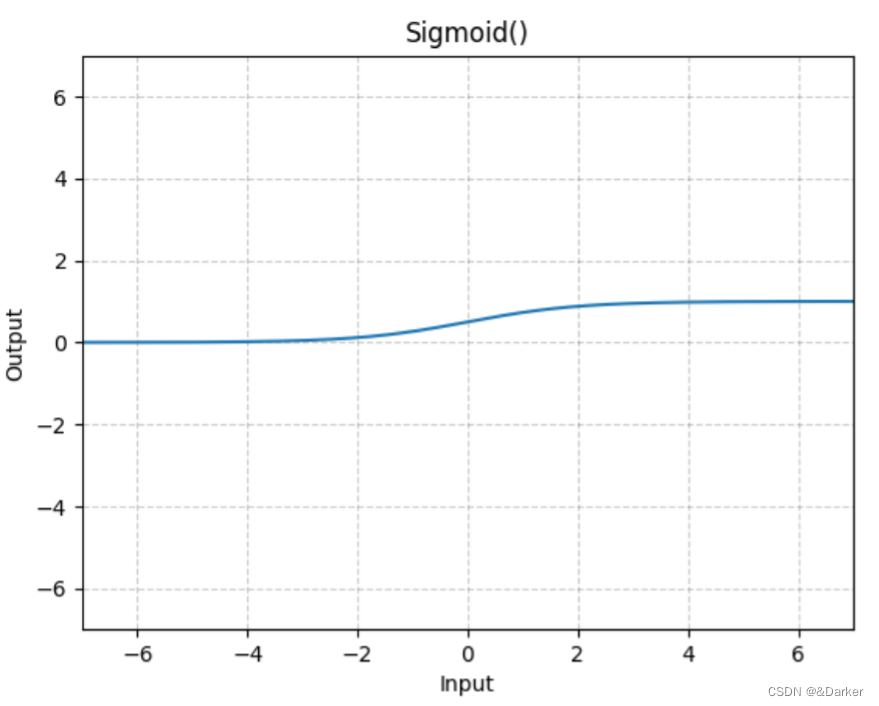
b.sigmoid:
$$Sigmoid(x)=\frac{1}{1+e^x}$$

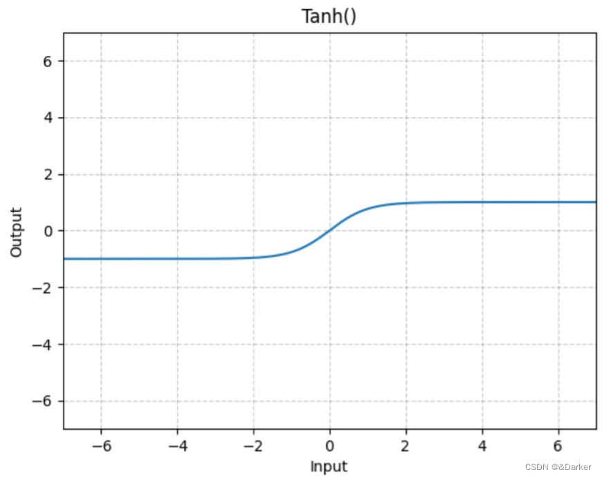
c.tanh:注意tanh可以理解是sigmoid的优化
$$Tabh(x)=\frac{e^x-e^{-x}}{e^x+e^{-x}}$$

d.softmax：该激活函数主要作用于分类任务，该函数映射之后的同一维度的元素之和为1
$$Softmax(x)=\frac{e^{x_i}}{{\sum }_{j=1}^n{e}^{x_j}}$$

e.gelu：是目前比较先进的激活函数
$$GELU(x)=0.5\ast x\ast (1+Tanh(\sqrt{\frac{2}{\pi }}\ast (x+0.044715\ast x^3)))$$

2.3.3 损失函数

概述：该函数主要的作用主要是用于计算预测值与真实值之间的差值，也就是模型的拟合效果；进而通过该函数计算梯度并更新权重，损失函数主要分为均方差损失函数以及交叉熵损失函数。

a. 均方差损失函数：主要用于求值类任务
$$loss=(预测值-真实值{)}^2$$
b.交叉熵损失函数：该函数主要用于分类任务的计算，在Pytorch框架中使用交叉熵损失函数CrossEntropyLoss其内部操作相当于使用了LogSoftmax+NLLLoss进行，下面展示交叉熵的计算逻辑
$$\begin{gathered} 现在有如下标准数据， \\ 元素\left[\begin{array}{ccc}1& 2& 3\\ 4& 5& 6\\ 7& 8& 9\end{array}\right];类别\left[\begin{array}{c}0\\ 1\\ 2\end{array}\right] \\ 交叉熵计算逻辑如下： \\ softmax计算：\left[\begin{array}{ccc}{a}_{11}=\frac{e^1}{e^1+e^2+e^3}& a_{12}=\frac{e^2}{e^1+e^2+e^3}& a_{13}=\frac{e^3}{e^1+e^2+e^3}\\ a_{21}=\frac{e^4}{e^4+e^5+e^6}& a_{22}=\frac{e^5}{e^4+e^5+e^6}& a_{23}=\frac{e^6}{e^4+e^5+e^6}\\ a_{31}=\frac{e^7}{e^7+e^8+e^9}& a_{32}=\frac{e^8}{e^7+e^8+e^9}& a_{33}=\frac{e^9}{e^7+e^8+e^9}\end{array}\right] \\ 元素第一行对应类别为第1个元素 \\ 元素第二行对应类别为第2个元素 \\ 元素第三行对于类别为第3个元素 \\ 损失函数计算：loss=\frac{-lo{g}_e(a_{11})+(-lo{g}_e(a_{22}))+(-lo{g}_e(a_{33}))}{3} \end{gathered}$$

2.4 训练模型实例

概述：如今有如下实例需要训练一个模型该模型的作用是输入一个五维向量，然后可以得到该五维最大值元素的位置。

i.e.:

[1,2,3,4,5] 最大值位置：4

[7,4,8,1,4] 最大值位置：2

[4,5,2,18,9] 最大值位置：3

…

"""
    训练一个模型实现效果：从一个随机5维向量中找出其中最大值的位置
    例如：
    [1,2,3,4,5]     5
    [9,2,3,6,5]     1
    [2,3,18,10,4]   3
    .....
"""
import numpy as np
import torch
import torch.nn as nn


# 生成随机五维向量
def build_sample():
    vector = np.random.random(5)
    return vector, np.argmax(vector)


def build_data(input_number):
    x_train = []
    y_train = []
    for i in range(input_number):
        x_t, y_t = build_sample()
        x_train.append(x_t)
        y_train.append(y_t)
    x_train = np.stack(x_train)
    y_train = np.stack(y_train)
    return torch.FloatTensor(x_train), torch.LongTensor(y_train)


# 构建模型:线性层，激活函数：softmax,损失函数：交叉熵
class TorchModel(nn.Module):
    def __init__(self, input_size):
        super(TorchModel, self).__init__()
        self.linear1 = nn.Linear(input_size, 20)
        self.linear2 = nn.Linear(20, 5)
        self.loss = nn.CrossEntropyLoss()

    def forward(self, x, y=None):
        y_temp = self.linear1(x)
        y_p = self.linear2(y_temp)
        y_pred = torch.nn.functional.softmax(y_p, dim=1)
        if y is not None:
            return self.loss(y_p, y)
        else:
            return y_pred


# 测试其模型准确度
def evaluate(model):
    # 获取测试数据
    x_eval, y_eval = build_data(100)
    # 模型预测
    model.eval()
    current = 0
    wrong = 0
    with torch.no_grad():
        result = model(x_eval)
        for y_e, res in zip(y_eval, result):
            if np.argmax(res) == y_e:
                current += 1
            else:
                wrong += 1

    return current/(current+wrong)

# 训练模型
def main():
    epoch_rounds = 1000         # 训练轮数
    train_number = 5000         # 总训练数据量
    input_size = 5              # 输入维度
    batch_size = 20             # 训练批次大小
    leaning_rate = 0.001        # 学习率
    # 定义模型
    model = TorchModel(input_size)
    # 定义优化器
    optim = torch.optim.Adam(model.parameters(), lr=leaning_rate)
    # 获取训练数据
    x_train, y_train = build_data(train_number)
    log = []
    flag = False
    # 训练模型
    for epoch_index in range(epoch_rounds):
        watch_loss = []
        for batch_index in range(train_number//batch_size):
            x_t = x_train[batch_index*batch_size:(batch_index+1)*batch_size]
            y_t = y_train[batch_index*batch_size:(batch_index+1)*batch_size]
            loss = model(x_t, y_t)      # 计算损失值
            loss.backward()             # 计算梯度
            optim.step()                # 更新权重
            optim.zero_grad()           # 梯度置零
            watch_loss.append(loss.item())
            if loss.item() < 0.01:
                flag = True
                break
        # 计算其模型准确率
        acc = evaluate(model)
        print("准确率：%f,损失值：%f" % (acc, np.mean(watch_loss)))
        log.append([acc, np.mean(watch_loss)])
        if flag:
            break
    # 保存模型
    torch.save(model.state_dict(), 'MaxModel.pt')


# 调用模型预测
def predict(model_path, input_vec):
    model = TorchModel(5)
    model.load_state_dict(torch.load(model_path))
    model.eval()
    with torch.no_grad():
        result = model(input_vec)
        for res, vec in zip(result, input_vec):
            print("输入：%s,最大值位置：%d" % (vec, np.argmax(res)))


if __name__=="__main__":
    # main()
    x_p, y_p = build_data(10)
    predict("MaxModel.pt", x_p)

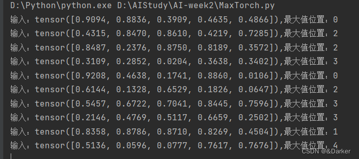
实现效果：

用模型预测
def predict(model_path, input_vec):
model = TorchModel(5)
model.load_state_dict(torch.load(model_path))
model.eval()
with torch.no_grad():
result = model(input_vec)
for res, vec in zip(result, input_vec):
print(“输入：%s,最大值位置：%d” % (vec, np.argmax(res)))

if name==“main”:
# main()
x_p, y_p = build_data(10)
predict(“MaxModel.pt”, x_p)
``
实现效果：