基于留学生实地调研的词频统计分析与词云可视化

Hi，大家好，我是半亩花海。本项目旨在通过解析 PDF 文档《留学生实地调研.pdf》，提取文本内容并进行词频统计和分析，生成热词柱状图和词云图，以便直观展示调研报告中的关键词及其出现频率。

---

目录

一、项目准备

1. PDF 文本数据选择

2. 遮罩底图选择

3. 环境配置

4. 每次生成可能需要更改的部分

三、项目内容

1. PDF 文档解析和文本提取

2. 文本分词和词频统计

3. 词频分析与可视化

4. 生成词云图

三、结果展示

1. 热词统计分析柱状图

2. 留学生词云统计图

四、完整代码

---

一、项目准备

1. PDF 文本数据选择

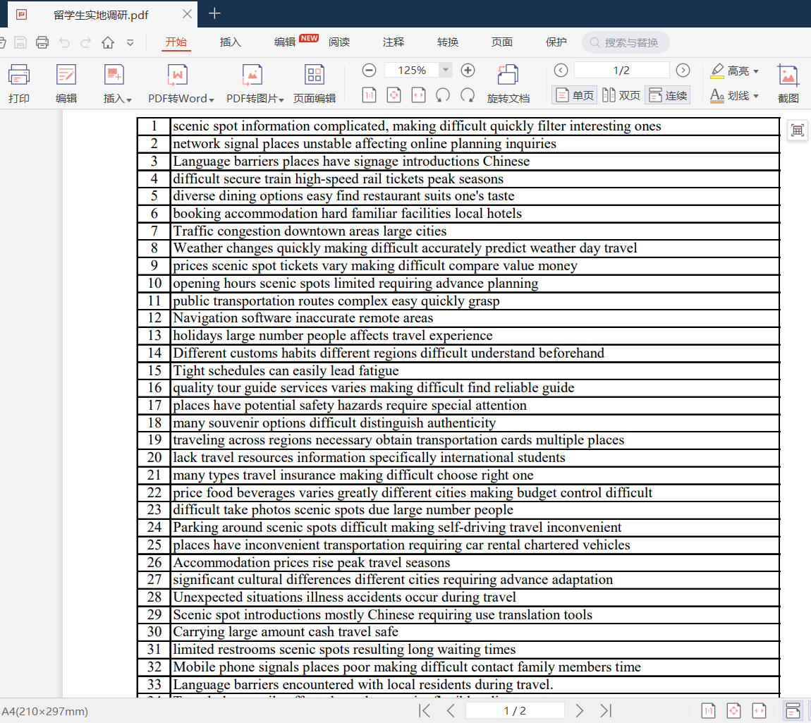
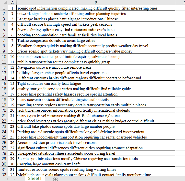
我选择的 PDF 文档由 Excel 文档转换而来，包含 100 条被调研的留学生的访谈记录，如下所示：

初始的Excel文档部分文本数据如下： 

注意：

数据处理的重要性：在生成词云图和热词统计分析过程中，数据的清洗和处理非常重要，尤其是中文文本处理中的分词和停用词过滤。

2. 遮罩底图选择

以下 tjzy.png 是我使用 PPT 绘制的摩天轮“天津之眼”的大致轮廓图，以此作为后续使用的遮罩图。

3. 环境配置

本项目使用的主要工具和库包括：

• pdfplumber：用于解析 PDF 文档。
• jieba：用于中文文本分词。
• WordCloud：用于生成词云图。
• numpy 和 matplotlib：用于数据处理和可视化。
• PIL (即 Pillow)：用于处理图像。

4. 每次生成可能需要更改的部分

每次需要基于同一个 PDF 文档再次生成词云图的时候，需要统一更改以下四个部分：

---

三、项目内容

1. PDF 文档解析和文本提取

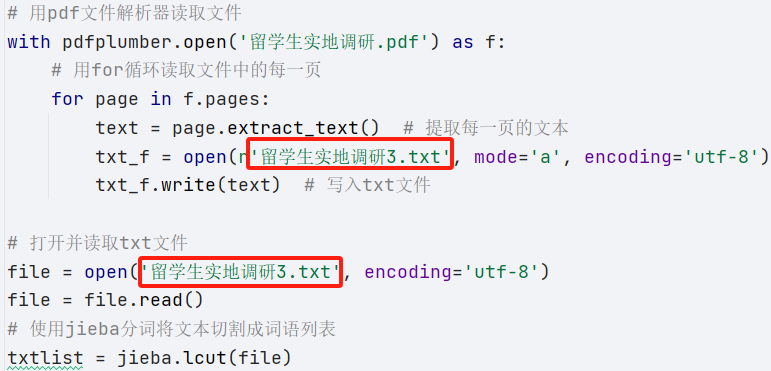
使用 pdfplumber 库读取 PDF 文档，并逐页提取文本，保存到一个 txt 文件中。

import pdfplumber

# 用pdf文件解析器读取文件
with pdfplumber.open('留学生实地调研.pdf') as f:
    # 用for循环读取文件中的每一页
    for page in f.pages:
        text = page.extract_text()  # 提取每一页的文本
        txt_f = open(r'留学生实地调研3.txt', mode='a', encoding='utf-8')  # 创建txt文件
        txt_f.write(text)  # 写入txt文件

2. 文本分词和词频统计

使用 jieba 库对提取的文本进行分词，并统计各词语的出现频率。

import jieba

file = open('留学生实地调研3.txt', encoding='utf-8')
file = file.read()
# 使用jieba分词将文本切割成词语列表
txtlist = jieba.lcut(file)
# 将分词后的词语列表用空格连接成字符串
string = " ".join(txtlist)

# 初始化停用词字典和词频统计字典
stop_words = {}
counts = {}
total_words = len(txtlist)  # 计算总词数

# 统计词频和单字词频（作为停用词）
for txt in txtlist:
    if len(txt) == 1:
        stop_words[txt] = stop_words.get(txt, 0) + 1
    else:
        counts[txt] = counts.get(txt, 0) + 1

3. 词频分析与可视化

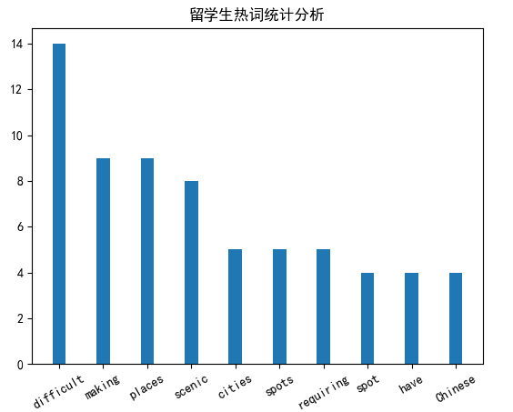
对词频数据进行排序，并输出前 10 个词语及其出现次数和频率。同时，使用 matplotlib 绘制热词柱状图。

import numpy as np
import matplotlib.pyplot as plt

# 对词频统计结果按出现次数排序
items = list(counts.items())
items.sort(key=lambda x: x[1], reverse=True)

# 输出前20个词语及其出现次数和出现频率
print("词语\t\t出现次数\t\t出现频率")
total_frequency = sum(count for word, count in items[:10])  # 前10个词语的总频率
for i in range(10):
    word, count = items[i]
    frequency = count / total_words * 100  # 计算词语出现频率
    relative_frequency = count / total_frequency * 100  # 计算词语相对频率
    print(f"{word}\t\t{count}\t\t{frequency:.2f}%\t\t{relative_frequency:.2f}%")

# 准备绘制柱状图的数据
y1 = []
labels = []
for i in range(1, 11):
    y1.append(items[i][1])  # 前10个词语的出现次数
    labels.append(items[i][0])  # 前10个词语的标签

# 绘制柱状图
width = 0.3
x = np.arange(len(y1))
a = [i for i in range(0, 10)]

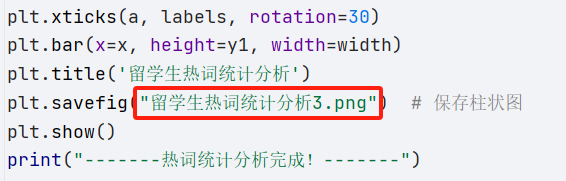
plt.xticks(a, labels, rotation=30)
plt.bar(x=x, height=y1, width=width)
plt.title('留学生热词统计分析')
plt.savefig("留学生热词统计分析3.png")  # 保存柱状图
plt.show()
print("-------热词统计分析完成！-------")

4. 生成词云图

使用 WordCloud 库生成词云图，并导出为图像文件。在生成词云图时采用了特定的遮罩图像 tjzy.png。遮罩图像的作用是控制词云图的形状，使其符合特定的视觉效果。使用 PIL 库加载遮罩图像，并将其传递给 WordCloud 对象，使生成的词云图在指定形状内填充。

from wordcloud import WordCloud
from PIL import Image

# 准备停用词列表
stoplist = []
item = list(stop_words.items())
for i in range(len(item)):
    txt, count = item[i]
    stoplist.append(txt)  # 将单字词语添加到停用词列表
setlist = set(stoplist)  # 转换为集合

# 加载所需的遮罩图像
mask = np.array(Image.open("tjzy.png"))

# 生成词云
wcd = WordCloud(width=1000, height=700, background_color='white', font_path='msyh.ttc', scale=15, stopwords=setlist, mask=mask)
wcd.generate(string)  # 根据文本生成词云
wcd.to_image()  # 转换为图像
print("-------热词词云生成完成！-------")

# 导出词云图像
wcd.to_file('留学生词云统计图3.png')

---

三、结果展示

1. 热词统计分析柱状图

此柱状图展示了前 10 个高频词语及其出现次数，便于直观了解调研报告中的重点词语。

2. 留学生词云统计图

此词云图展示了调研报告中的词语，以词语出现频率大小为依据，词频越高，词语显示越大。

---

四、完整代码

#!/usr/bin/env python
# -*- coding:utf-8 -*-
"""
@File    : 词云图.py
@IDE     : PyCharm
@Author  : 半亩花海
@Date    : 2024/05/21 16:31
"""
import pdfplumber
import jieba
from wordcloud import WordCloud
import numpy as np
import matplotlib.pyplot as plt
from PIL import Image

plt.rcParams['font.sans-serif'] = ['SimHei']
plt.rcParams['axes.unicode_minus'] = False

# 用pdf文件解析器读取文件
with pdfplumber.open('留学生实地调研.pdf') as f:
    # 用for循环读取文件中的每一页
    for page in f.pages:
        text = page.extract_text()  # 提取每一页的文本
        txt_f = open(r'留学生实地调研3.txt', mode='a', encoding='utf-8')  # 创建txt文件
        txt_f.write(text)  # 写入txt文件

# 打开并读取txt文件
file = open('留学生实地调研3.txt', encoding='utf-8')
file = file.read()
# 使用jieba分词将文本切割成词语列表
txtlist = jieba.lcut(file)
# 将分词后的词语列表用空格连接成字符串
string = " ".join(txtlist)

# 初始化停用词字典和词频统计字典
stop_words = {}
counts = {}
total_words = len(txtlist)  # 计算总词数

# 统计词频和单字词频（作为停用词）
for txt in txtlist:
    if len(txt) == 1:
        stop_words[txt] = stop_words.get(txt, 0) + 1
    else:
        counts[txt] = counts.get(txt, 0) + 1

# 对词频统计结果按出现次数排序
items = list(counts.items())
items.sort(key=lambda x: x[1], reverse=True)

# 输出前20个词语及其出现次数和出现频率
print("词语\t\t出现次数\t\t出现频率")
total_frequency = sum(count for word, count in items[:10])  # 前10个词语的总频率
for i in range(10):
    word, count = items[i]
    frequency = count / total_words * 100  # 计算词语出现频率
    relative_frequency = count / total_frequency * 100  # 计算词语相对频率
    print(f"{word}\t\t{count}\t\t{frequency:.2f}%\t\t{relative_frequency:.2f}%")

# 准备绘制柱状图的数据
y1 = []
labels = []
for i in range(1, 11):
    y1.append(items[i][1])  # 前10个词语的出现次数
    labels.append(items[i][0])  # 前10个词语的标签

# 绘制柱状图
width = 0.3
x = np.arange(len(y1))
a = [i for i in range(0, 10)]

plt.xticks(a, labels, rotation=30)
plt.bar(x=x, height=y1, width=width)
plt.title('留学生热词统计分析')
plt.savefig("留学生热词统计分析3.png")  # 保存柱状图
plt.show()
print("-------热词统计分析完成！-------")

# 准备停用词列表
stoplist = []
item = list(stop_words.items())
for i in range(len(item)):
    txt, count = item[i]
    stoplist.append(txt)  # 将单字词语添加到停用词列表
setlist = set(stoplist)  # 转换为集合

# 加载所需的遮罩图像
mask = np.array(Image.open("tjzy.png"))

# 生成词云
wcd = WordCloud(width=1000, height=700, background_color='white', font_path='msyh.ttc', scale=15, stopwords=setlist, mask=mask)
wcd.generate(string)  # 根据文本生成词云
wcd.to_image()  # 转换为图像
print("-------热词词云生成完成！-------")

# 导出词云图像
wcd.to_file('留学生词云统计图3.png')