


线性回归
模型公式:
p
r
i
c
e
=
w
a
r
e
a
⋅
a
r
e
a
+
w
a
g
e
⋅
a
g
e
+
b
\mathrm{price} = w_{\mathrm{area}} \cdot \mathrm{area} + w_{\mathrm{age}} \cdot \mathrm{age} + b
price=warea⋅area+wage⋅age+b
- 神经网络中的单个神经元的一部分就是这个公式,只不过在此基础上添加了sigmoid函数
损失函数
L ( w , b ) = 1 n ∑ i = 1 n l ( i ) ( w , b ) = 1 n ∑ i = 1 n 1 2 ( w ⊤ x ( i ) + b − y ( i ) ) 2 . L(\mathbf{w}, b) =\frac{1}{n}\sum_{i=1}^n l^{(i)}(\mathbf{w}, b) =\frac{1}{n} \sum_{i=1}^n \frac{1}{2}\left(\mathbf{w}^\top \mathbf{x}^{(i)} + b - y^{(i)}\right)^2. L(w,b)=n1i=1∑nl(i)(w,b)=n1i=1∑n21(w⊤x(i)+b−y(i))2.
手动实现
w = torch.tensor(np.random.normal(0, 0.01, (num_inputs, 1)), dtype=torch.float32)
b = torch.zeros(1, dtype=torch.float32)

w.requires_grad_(requires_grad=True)
b.requires_grad_(requires_grad=True)
定义变量为tensor
def linreg(X, w, b):
    return torch.mm(X, w) + b
定义模型
def squared_loss(y_hat, y):
    return (y_hat - y.view(y_hat.size())) ** 2 / 2
损失函数
def sgd(params, lr, batch_size):
    for param in params:
        param.data -= lr * param.grad / batch_size # ues .data to operate param without gradient track
定义优化迭代函数
# super parameters init
lr = 0.03
num_epochs = 5

net = linreg
loss = squared_loss

# training
for epoch in range(num_epochs):  # training repeats num_epochs times
    # in each epoch, all the samples in dataset will be used once

    # X is the feature and y is the label of a batch sample
    for X, y in data_iter(batch_size, features, labels):
        l = loss(net(X, w, b), y).sum()
        # calculate the gradient of batch sample loss
        l.backward()
        # using small batch random gradient descent to iter model parameters
        sgd([w, b], lr, batch_size)
        # reset parameter gradient
        w.grad.data.zero_()
        b.grad.data.zero_()
    train_l = loss(net(features, w, b), labels)
    print('epoch %d, loss %f' % (epoch + 1, train_l.mean().item()))
训练步骤
使用Pytorch模型来定义网络
class LinearNet(nn.Module):
    def __init__(self, n_feature):
        super(LinearNet, self).__init__()      # call father function to init
        self.linear = nn.Linear(n_feature, 1)  # function prototype: `torch.nn.Linear(in_features, out_features, bias=True)`

    def forward(self, x):
        y = self.linear(x)
        return y
自定义网络层的经典模板
# method one
net = nn.Sequential(
    nn.Linear(num_inputs, 1)
    # other layers can be added here
    )

# method two
net = nn.Sequential()
net.add_module('linear', nn.Linear(num_inputs, 1))
# net.add_module ......

# method three
from collections import OrderedDict
net = nn.Sequential(OrderedDict([
          ('linear', nn.Linear(num_inputs, 1))
          # ......
        ]))
三种组合网络的经典结构
softmax
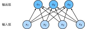
o 1 , o 2 , o 3 o_1, o_2, o_3 o1,o2,o3分别是三个类别的factor,最后需要转换为概率。
y ^ 1 = exp ( o 1 ) ∑ i = 1 3 exp ( o i ) , y ^ 2 = exp ( o 2 ) ∑ i = 1 3 exp ( o i ) , y ^ 3 = exp ( o 3 ) ∑ i = 1 3 exp ( o i ) . \hat{y}1 = \frac{ \exp(o_1)}{\sum_{i=1}^3 \exp(o_i)},\quad \hat{y}2 = \frac{ \exp(o_2)}{\sum_{i=1}^3 \exp(o_i)},\quad \hat{y}3 = \frac{ \exp(o_3)}{\sum_{i=1}^3 \exp(o_i)}. y^1=∑i=13exp(oi)exp(o1),y^2=∑i=13exp(oi)exp(o2),y^3=∑i=13exp(oi)exp(o3).
分别表示三种类别的概率
交叉熵损失函数
- 之前用的平方损失不能很好的评价分类结果,例如 y ^ 1 ( i ) = y ^ 2 ( i ) = 0.2 \hat y^{(i)}_1=\hat y^{(i)}_2=0.2 y^1(i)=y^2(i)=0.2比 y ^ 1 ( i ) = 0 , y ^ 2 ( i ) = 0.4 \hat y^{(i)}_1=0, \hat y^{(i)}_2=0.4 y^1(i)=0,y^2(i)=0.4的损失要小很多,虽然两者都有同样正确的分类预测结果。这主要是因为把误分类的情况也考虑进去了。
- 交叉熵损失函数简化了,只评价正分类的结果。 H ( y ( i ) , y ^ ( i ) ) = − log y ^ y ( i ) ( i ) H(\boldsymbol y^{(i)}, \boldsymbol {\hat y}^{(i)}) = -\log \hat y_{y^{(i)}}^{(i)} H(y(i),y^(i))=−logy^y(i)(i)。其中 y ^ y ( i ) ( i ) \hat y_{y^{(i)}}^{(i)} y^y(i)(i)表示模型把输入判定为类别i的概率,而i是ground truth,也就是正确分类的概率。
- 为了矢量化计算方便,交叉熵的公式如下:
H ( y ( i ) , y ^ ( i ) ) = − ∑ j = 1 q y j ( i ) log y ^ j ( i ) , H\left(\boldsymbol y^{(i)}, \boldsymbol {\hat y}^{(i)}\right ) = -\sum_{j=1}^q y_j^{(i)} \log \hat y_j^{(i)}, H(y(i),y^(i))=−j=1∑qyj(i)logy^j(i),
多层感知机

- 在线性回归的基础上增加了激活函数,层数
- 经典激活函数有ReLU, sigmoid, tanh
ReLU函数

- 对应的函数导数

sigmoid 函数
sigmoid ( x ) = 1 1 + exp ( − x ) . \text{sigmoid}(x) = \frac{1}{1 + \exp(-x)}. sigmoid(x)=1+exp(−x)1.

-
对应的函数导数图像

-
Sigmoid 的梯度随着结果接近1, -1而急剧减小,意味着在训练的后期会出现“训不动”的现象。相比之下ReLU的梯度一直很稳。对于这个问题Baidu提出过一种方法,在模型训练的而后期,手动增加前面节点的learning rate, 防止update step 淹没。
-
tanh函数结构与sigmoid很相似
tanh ( x ) = 1 − exp ( − 2 x ) 1 + exp ( − 2 x ) . \text{tanh}(x) = \frac{1 - \exp(-2x)}{1 + \exp(-2x)}. tanh(x)=1+exp(−2x)1−exp(−2x).


 733
733


 被折叠的 条评论
为什么被折叠?
被折叠的 条评论
为什么被折叠?
 到【灌水乐园】发言


