Python数据分析示例（1）Day2

最新推荐文章于 2024-05-12 10:00:00 发布

图图酱

最新推荐文章于 2024-05-12 10:00:00 发布

阅读量1.1w

点赞数 1

分类专栏： Python数据处理

本文链接：https://blog.csdn.net/u010456562/article/details/51332995

版权

Python数据处理专栏收录该内容

14 篇文章 3 订阅

订阅专栏

说明：本文章为Python数据处理学习日志，主要内容来自书本《利用Python进行数据分析》，Wes McKinney著，机械工业出版社。

“以我的观点来看，如果只需要用Python进行高效的数据分析工作，根本就没必要非得成为通用软件编程方面的专家不可。”——作者

接下来是书本一些代码的实现，用来初步了解Python处理数据的功能，相关资源可在下方链接下载。
书本相关资源

读取文件第一行

相关例子可以再shell中执行，也可以再Canopy Editor中执行。以下代码在Canopy Editor中执行。

path='E:\\Enthought\\book\\ch02\\usagov_bitly_data2012-03-16-1331923249.txt'
open(path).readline()

在shell中执行则不要转置符’\’，path为存放文件路径。在shell中执行一定要用pylab模式打开，不然绘图会出现些小问题。

path='E:\Enthought\book\ch02\usagov_bitly_data2012-03-16-1331923249.txt'

输出结果：

Out[2]: '{ "a": "Mozilla\\/5.0 (Windows NT 6.1; WOW64) AppleWebKit\\/535.11 (KHTML, like Gecko) Chrome\\/17.0.963.78 Safari\\/535.11", "c": "US", "nk": 1, "tz": "America\\/New_York", "gr": "MA", "g": "A6qOVH", "h": "wfLQtf", "l": "orofrog", "al": "en-US,en;q=0.8", "hh": "1.usa.gov", "r": "http:\\/\\/www.facebook.com\\/l\\/7AQEFzjSi\\/1.usa.gov\\/wfLQtf", "u": "http:\\/\\/www.ncbi.nlm.nih.gov\\/pubmed\\/22415991", "t": 1331923247, "hc": 1331822918, "cy": "Danvers", "ll": [ 42.576698, -70.954903 ] }\n'

以上结果为纯文本加载。
Python中的内置或者第三方模块将JSON字符串转化为Python字典对象。这里，将使用json模块及其loads函数逐行加载已经下载好的数据文件：

import json
path='E:\\Enthought\\book\\ch02\\usagov_bitly_data2012-03-16-1331923249.txt'
records=[json.loads(line) for line in open(path)]
records[0]

这样，records对象就成了一组Python字典了。

Out[6]: 
{u'a': u'Mozilla/5.0 (Windows NT 6.1; WOW64) AppleWebKit/535.11 (KHTML, like Gecko) Chrome/17.0.963.78 Safari/535.11',
 u'al': u'en-US,en;q=0.8',
 u'c': u'US',
 u'cy': u'Danvers',
 u'g': u'A6qOVH',
 u'gr': u'MA',
 u'h': u'wfLQtf',
 u'hc': 1331822918,
 u'hh': u'1.usa.gov',
 u'l': u'orofrog',
 u'll': [42.576698, -70.954903],
 u'nk': 1,
 u'r': u'http://www.facebook.com/l/7AQEFzjSi/1.usa.gov/wfLQtf',
 u't': 1331923247,
 u'tz': u'America/New_York',
 u'u': u'http://www.ncbi.nlm.nih.gov/pubmed/22415991'}

现在，只要一字符串形式给出想要访问的键就可以得到当前记录中相应的值了：

records[0]['tz']
Out[7]: u'America/New_York'

print records[0]['tz']
America/New_York

对时区进行计数

1.用纯Python对时区进行计数

假设我们想知道该数据集中最常出现的是哪个时区（即tz字段）。首先，我们用列表推导式取出一组时区：

time_zones=[rec['tz'] for rec in records if 'tz' in rec]
time_zones[:10] #获取前10条记录的tz

结果：

Out[12]: 
[u'America/New_York',
 u'America/Denver',
 u'America/New_York',
 u'America/Sao_Paulo',
 u'America/New_York',
 u'America/New_York',
 u'Europe/Warsaw',
 u'',
 u'',
 u'']

接下来对时区进行计数：

 def get_counts(sequence):
    counts={}
    for x in sequence:
        if x in counts:
            counts[x]+=1
        else:
            counts[x]=1
    return counts

或者使用Python标准库

def get_counts2(sequence):
    counts=defaultdict(int) #所有初始值均会初始化为0
    for x in sequence:
        counts[x]+=1
    return counts

调用函数

counts = get_counts(time_zones)

counts['America/New_York']
Out[20]: 1251

len(time_zones)
Out[21]: 3440

如果只想要得到前10位的时区及其计数值，我们需要用到一些关羽字典的处理技巧：

def top_counts(count_dict,n=10):
    value_key_pairs=[(count,tz) for tz,count in count_dict.items()]
    value_key_pairs.sort()
    return value_key_pairs[-n:]

数据处理结果

top_counts(counts)
Out[26]: 
[(33, u'America/Sao_Paulo'),
 (35, u'Europe/Madrid'),
 (36, u'Pacific/Honolulu'),
 (37, u'Asia/Tokyo'),
 (74, u'Europe/London'),
 (191, u'America/Denver'),
 (382, u'America/Los_Angeles'),
 (400, u'America/Chicago'),
 (521, u''),
 (1251, u'America/New_York')]

或者在Python标准库中找到collections.Counter类，处理起来就比较简单：

from collections import Counter
counts=Counter(time_zones)
counts.most_common(10)
Out[29]: 
[(u'America/New_York', 1251),
 (u'', 521),
 (u'America/Chicago', 400),
 (u'America/Los_Angeles', 382),
 (u'America/Denver', 191),
 (u'Europe/London', 74),
 (u'Asia/Tokyo', 37),
 (u'Pacific/Honolulu', 36),
 (u'Europe/Madrid', 35),
 (u'America/Sao_Paulo', 33)]

2.用pandas对时区进行计数

DataFrame是pandas中重要的数据结构，它用于将数据表示成一个表格。

from pandas import DataFrame,Series
import pandas as pd;import numpy as np
frame = DataFrame(records)

结果

frame['tz'][:10]
Out[34]: 
0     America/New_York
1       America/Denver
2     America/New_York
3    America/Sao_Paulo
4     America/New_York
5     America/New_York
6        Europe/Warsaw
7                     
8                     
9                     
Name: tz, dtype: object

frame[‘tz’]所返回的Series对象有一个value_counts方法，该方法可以让我们得到所需要的信息：

tz_counts = frame['tz'].value_counts()
tz_counts[:10]
Out[36]: 
America/New_York       1251
                        521
America/Chicago         400
America/Los_Angeles     382
America/Denver          191
Europe/London            74
Asia/Tokyo               37
Pacific/Honolulu         36
Europe/Madrid            35
America/Sao_Paulo        33
Name: tz, dtype: int64

绘图

然后，我们可以利用绘图库（即matplotlib）为该段数据生成一张图片。为此，我们先给记录中位未知或者缺失的时区填上一个替代值。fillna函数可以替换缺失值（NA），而未知值（空字符串）则可以通过布尔型数组索引加以替换：

clean_tz=frame['tz'].fillna('Missing')
clean_tz[clean_tz==''] = 'Unknown'
tz_counts=clean_tz.value_counts()
tz_counts[:10]
Out[41]: 
America/New_York       1251
Unknown                 521
America/Chicago         400
America/Los_Angeles     382
America/Denver          191
Missing                 120
Europe/London            74
Asia/Tokyo               37
Pacific/Honolulu         36
Europe/Madrid            35
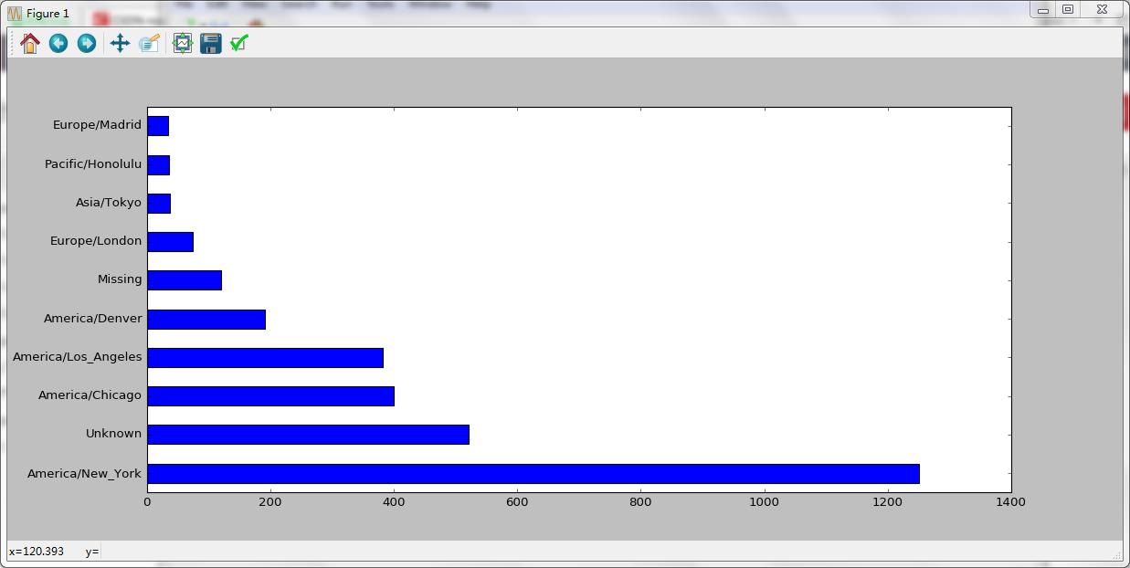
Name: tz, dtype: int64

绘图

tz_counts[:10].plot(kind='barh',rot=0)
Out[42]: <matplotlib.axes._subplots.AxesSubplot at 0xe50b1d0>

结果
示例数据中最常出现的时区

对Agent(‘a’)进行划分

‘a’字段含有执行URL缩短操作的浏览器、设备、应用程序的相关信息：

frame['a'][0]
Out[43]: u'Mozilla/5.0 (Windows NT 6.1; WOW64) AppleWebKit/535.11 (KHTML, like Gecko) Chrome/17.0.963.78 Safari/535.11'

运用Python内置的字符串函数和正则表达式，可以将这种字符串的第一节（与浏览器大致对应）分离出来并得到另外一份用户行为摘要：

results = Series([x.split()[0] for x in frame.a.dropna()]) #按空格切分字段'a'
results[:5]
Out[45]: 
0               Mozilla/5.0
1    GoogleMaps/RochesterNY
2               Mozilla/4.0
3               Mozilla/5.0
4               Mozilla/5.0
dtype: object
results.value_counts()[:8]
Out[46]: 
Mozilla/5.0                 2594
Mozilla/4.0                  601
GoogleMaps/RochesterNY       121
Opera/9.80                    34
TEST_INTERNET_AGENT           24
GoogleProducer                21
Mozilla/6.0                    5
BlackBerry8520/5.0.0.681       4
dtype: int64

现在，根据Windows用户和非Windows用户对时区统计信息进行分解。为了方便起见，嘉定只要agent字符串中含有“Windows”就认为该用户为Windows用户。

cframe = frame[frame.a.notnull()] #删除agent为空的记录
 operating_system = np.where(cframe['a'].str.contains('Windows'),'Windows','Not Windows')
operating_system[:5]
Out[52]: #可能是版本原因，此处略有不同，原书以frame形式输出
array(['Windows', 'Not Windows', 'Windows', 'Not Windows', 'Windows'], 
      dtype='|S11')

接下来就可以根据时区和新得到的操作系统列表对数据进行分组，然后通过size对分组结果进行计数（类似于上面的value_counts函数），并利用unstack对技术结果进行重塑：

by_tz_os = cframe.groupby(['tz',operating_system])
agg_counts = by_tz_os.size().unstack().fillna(0)
agg_counts[:10]
Out[56]: 
                                Not Windows  Windows
tz                                                  
                                      245.0    276.0
Africa/Cairo                            0.0      3.0
Africa/Casablanca                       0.0      1.0
Africa/Ceuta                            0.0      2.0
Africa/Johannesburg                     0.0      1.0
Africa/Lusaka                           0.0      1.0
America/Anchorage                       4.0      1.0
America/Argentina/Buenos_Aires          1.0      0.0
America/Argentina/Cordoba               0.0      1.0
America/Argentina/Mendoza               0.0      1.0

最后，选出最常出现的时区。根据agg_counts中的行数构造一个间接索引数组：

indexer = agg_counts.sum(1).argsort()
indexer[:10]
Out[58]: 
tz
                                  24
Africa/Cairo                      20
Africa/Casablanca                 21
Africa/Ceuta                      92
Africa/Johannesburg               87
Africa/Lusaka                     53
America/Anchorage                 54
America/Argentina/Buenos_Aires    57
America/Argentina/Cordoba         26
America/Argentina/Mendoza         55
dtype: int64

然后通过take按照这个顺序截取最后10行：

count_subset = agg_counts.take(indexer)[-10:]
count_subset
Out[60]: 
                     Not Windows  Windows
tz                                       
America/Sao_Paulo           13.0     20.0
Europe/Madrid               16.0     19.0
Pacific/Honolulu             0.0     36.0
Asia/Tokyo                   2.0     35.0
Europe/London               43.0     31.0
America/Denver             132.0     59.0
America/Los_Angeles        130.0    252.0
America/Chicago            115.0    285.0
                           245.0    276.0
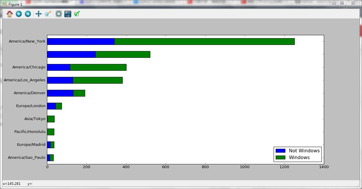
America/New_York           339.0    912.0

生成图形

count_subset.plot(kind='barh',stacked=True)
Out[61]: <matplotlib.axes._subplots.AxesSubplot at 0xeb89d68>

结果

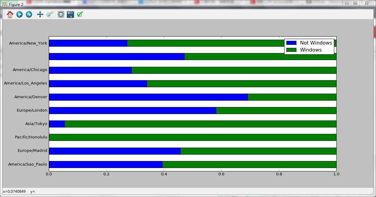
为了看清楚小分组中Windows用户的相对比例，可以将各行规范化为“总计为1”并重新绘图：

normed_subset = count_subset.div(count_subset.sum(1),axis=0)
normed_subset.plot(kind='barh',stacked=True)
Out[63]: <matplotlib.axes._subplots.AxesSubplot at 0xed1e1d0>

结果

图图酱

关注

1
点赞
踩
12

收藏

觉得还不错? 一键收藏
3
评论
Python数据分析示例（1）Day2

说明：本文章为Python数据处理学习日志，主要内容来自书本《利用Python进行数据分析》，Wes McKinney著，机械工业出版社。“以我的观点来看，如果只需要用Python进行高效的数据分析工作，根本就没必要非得成为通用软件编程方面的专家不可。”——作者接下来是书本一些代码的实现，用来初步了解Python处理数据的功能，相关资源可在下方链接下载。书本相关资源读取文件第一行相关例子可以再s
复制链接

扫一扫