【深度学习-吴恩达】L1-3 浅层神经网络 作业

L1 深度学习概论

3 浅层神经网络

作业链接：吴恩达《深度学习》 - Heywhale.com

0 作业任务

用1层隐藏层的神经网络分类二维数据

目标：

• 实现具有单个隐藏层的2分类神经网络

• 使用具有非线性激活函数的神经元

• 计算交叉熵损失

• 实现前向和后向传播

1 Logistic回归二分类的实现

1.1 导入安装包

• numpy是Python科学计算的基本包。
• sklearn提供了用于数据挖掘和分析的简单有效的工具。
• matplotlib是在Python中常用的绘制图形的库。
• testCases提供了一些测试示例用以评估函数的正确性
• planar_utils提供了此作业中使用的各种函数

# Package imports
import numpy as np
import matplotlib.pyplot as plt
from testCases import *
import sklearn
import sklearn.datasets
import sklearn.linear_model
from planar_utils import plot_decision_boundary, sigmoid, load_planar_dataset, load_extra_datasets

%matplotlib inline

np.random.seed(1) # set a seed so that the results are consistent

1.2 导入数据集

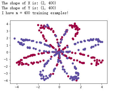
X, Y = load_planar_dataset() 
# Visualize the data:
plt.scatter(X[0, :], X[1, :], c=Y.reshape(X[0,:].shape), s=40, cmap=plt.cm.Spectral)

shape_X = X.shape
shape_Y = Y.shape

m = shape_X[1]  # training set size

print ('The shape of X is: ' + str(shape_X))
print ('The shape of Y is: ' + str(shape_Y))
print ('I have m = %d training examples!' % (m))

得到数据集：

• X形状为(2, 400)
• Y形状为(1, 400)
• 一共有m个输入数据

如下图所示：

1.3 简单的Logistic回归

使用sklearn内置函数执行

# Train the logistic regression classifier
clf = sklearn.linear_model.LogisticRegressionCV();
clf.fit(X.T, Y.T);
# Plot the decision boundary for logistic regression
plot_decision_boundary(lambda x: clf.predict(x), X, Y)
plt.title("Logistic Regression")
# Print accuracy
LR_predictions = clf.predict(X.T)
print ('Accuracy of logistic regression: %d ' % float((np.dot(Y,LR_predictions) + np.dot(1-Y,1-LR_predictions))/float(Y.size)*100) +
       '% ' + "(percentage of correctly labelled datapoints)")

得到结果如下所示：

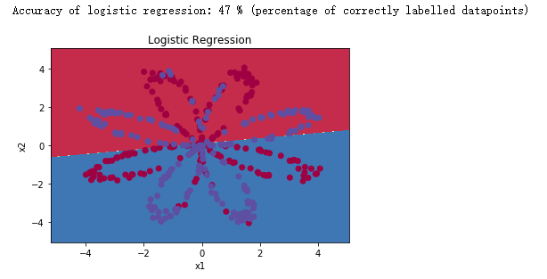
由于数据集不是线性可分的，因此逻辑回归效果不佳

• 注意这里出现bug，需要将planar_utils.py文件中的plt.scatter函数修改为：

  plt.scatter(X[0, :], X[1, :], c=np.squeeze(y), cmap=plt.cm.Spectral)
  

2 神经网络二分类的实现

2.1 定义神经网络结构

练习：定义三个变量：

• n_x：输入层的大小
• n_h：隐藏层的大小
• n_y：输出层的大小

# GRADED FUNCTION: layer_sizes

def layer_sizes(X, Y):
    """
    Arguments:
    X -- input dataset of shape (input size, number of examples)
    Y -- labels of shape (output size, number of examples)
    
    Returns:
    n_x -- the size of the input layer
    n_h -- the size of the hidden layer
    n_y -- the size of the output layer
    """
    n_x = X.shape[0] # size of input layer
    n_h = 4
    n_y = Y.shape[0] # size of output layer

    return (n_x, n_h, n_y)

2.2 初始化模型的参数

练习：实现函数 initialize_parameters()。

# GRADED FUNCTION: initialize_parameters

def initialize_parameters(n_x, n_h, n_y):
    """
    Argument:
    n_x -- size of the input layer
    n_h -- size of the hidden layer
    n_y -- size of the output layer
    
    Returns:
    params -- python dictionary containing your parameters:
                    W1 -- weight matrix of shape (n_h, n_x)
                    b1 -- bias vector of shape (n_h, 1)
                    W2 -- weight matrix of shape (n_y, n_h)
                    b2 -- bias vector of shape (n_y, 1)
    """
    
    np.random.seed(2) # we set up a seed so that your output matches ours although the initialization is random.
    
    W1 = np.random.randn(n_h,n_x) * 0.01
    b1 = np.zeros((n_h,1))
    W2 = np.random.randn(n_y,n_h) * 0.01
    b2 = np.zeros((n_y,1))
    
    assert (W1.shape == (n_h, n_x))
    assert (b1.shape == (n_h, 1))
    assert (W2.shape == (n_y, n_h))
    assert (b2.shape == (n_y, 1))
    
    parameters = {"W1": W1,
                  "b1": b1,
                  "W2": W2,
                  "b2": b2}
    
    return parameters

• 将权重矩阵初始化为随机数
• 将偏差向量初始化为0

2.3 循环

练习：实现forward_propagation（）。

# GRADED FUNCTION: forward_propagation

def forward_propagation(X, parameters):
    """
    Argument:
    X -- input data of size (n_x, m)
    parameters -- python dictionary containing your parameters (output of initialization function)
    
    Returns:
    A2 -- The sigmoid output of the second activation
    cache -- a dictionary containing "Z1", "A1", "Z2" and "A2"
    """
    # Retrieve each parameter from the dictionary "parameters"
    W1 = parameters["W1"]
    b1 = parameters["b1"]
    W2 = parameters["W2"]
    b2 = parameters["b2"]
    
    # Implement Forward Propagation to calculate A2 (probabilities)
    Z1 = np.dot(W1,X) + b1
    A1 = np.tanh(Z1)
    Z2 = np.dot(W2,A1) + b2
    A2 = sigmoid(Z2)
    
    assert(A2.shape == (1, X.shape[1]))
    
    cache = {"Z1": Z1,
             "A1": A1,
             "Z2": Z2,
             "A2": A2}
    
    return A2, cache

• 第一层激活函数使用tanh函数
• 第二层激活函数使用sigmoid函数

练习：实现compute_cost（）以计算损失$J$的值。

# GRADED FUNCTION: compute_cost

def compute_cost(A2, Y, parameters):
    """
    Computes the cross-entropy cost given in equation (13)
    
    Arguments:
    A2 -- The sigmoid output of the second activation, of shape (1, number of examples)
    Y -- "true" labels vector of shape (1, number of examples)
    parameters -- python dictionary containing your parameters W1, b1, W2 and b2
    
    Returns:
    cost -- cross-entropy cost given equation (13)
    """
    
    m = Y.shape[1] # number of example

    # Compute the cross-entropy cost
    logprobs = Y*np.log(A2) + (1-Y)* np.log(1-A2)
    cost = -1/m * np.sum(logprobs)
    
    cost = np.squeeze(cost)
    # makes sure cost is the dimension we expect. 
    # E.g., turns [[17]] into 17 
    assert(isinstance(cost, float))
    
    return cost

练习：实现函数backward_propagation（）

# GRADED FUNCTION: backward_propagation

def backward_propagation(parameters, cache, X, Y):
    """
    Implement the backward propagation using the instructions above.
    
    Arguments:
    parameters -- python dictionary containing our parameters 
    cache -- a dictionary containing "Z1", "A1", "Z2" and "A2".
    X -- input data of shape (2, number of examples)
    Y -- "true" labels vector of shape (1, number of examples)
    
    Returns:
    grads -- python dictionary containing your gradients with respect to different parameters
    """
    m = X.shape[1]
    
    # First, retrieve W1 and W2 from the dictionary "parameters".
    W1 = parameters["W1"]
    W2 = parameters["W2"]
        
    # Retrieve also A1 and A2 from dictionary "cache".
    A1 = cache["A1"]
    A2 = cache["A2"]
    
    # Backward propagation: calculate dW1, db1, dW2, db2. 
    dZ2= A2 - Y
    dW2 = 1 / m * np.dot(dZ2,A1.T)
    db2 = 1 / m * np.sum(dZ2,axis=1,keepdims=True)
    dZ1 = np.dot(W2.T,dZ2) * (1-np.power(A1,2))
    dW1 = 1 / m * np.dot(dZ1,X.T)
    db1 = 1 / m * np.sum(dZ1,axis=1,keepdims=True)
    
    grads = {"dW1": dW1,
             "db1": db1,
             "dW2": dW2,
             "db2": db2}
    
    return grads

练习：实现参数更新。 使用梯度下降，你必须使用（dW1，db1，dW2，db2）才能更新（W1，b1，W2，b2）。

# GRADED FUNCTION: update_parameters

def update_parameters(parameters, grads, learning_rate = 1.2):
    """
    Updates parameters using the gradient descent update rule given above
    
    Arguments:
    parameters -- python dictionary containing your parameters 
    grads -- python dictionary containing your gradients 
    
    Returns:
    parameters -- python dictionary containing your updated parameters 
    """
    # Retrieve each parameter from the dictionary "parameters"
    W1 = parameters["W1"]
    b1 = parameters["b1"]
    W2 = parameters["W2"]
    b2 = parameters["b2"]
    
    # Retrieve each gradient from the dictionary "grads"
    dW1 = grads["dW1"]
    db1 = grads["db1"]
    dW2 = grads["dW2"]
    db2 = grads["db2"]
    
    # Update rule for each parameter
    W1 = W1 - learning_rate * dW1
    b1 = b1 - learning_rate * db1
    W2 = W2 - learning_rate * dW2
    b2 = b2 - learning_rate * db2
    
    parameters = {"W1": W1,
                  "b1": b1,
                  "W2": W2,
                  "b2": b2}
    
    return parameters

2.4 集成函数

练习：在nn_model（）中建立你的神经网络模型。

def nn_model(X, Y, n_h, num_iterations = 10000, print_cost=False):
    """
    Arguments:
    X -- dataset of shape (2, number of examples)
    Y -- labels of shape (1, number of examples)
    n_h -- size of the hidden layer
    num_iterations -- Number of iterations in gradient descent loop
    print_cost -- if True, print the cost every 1000 iterations
    
    Returns:
    parameters -- parameters learnt by the model. They can then be used to predict.
    """
    
    np.random.seed(3)
    n_x = layer_sizes(X, Y)[0]
    n_y = layer_sizes(X, Y)[2]
    
    # Initialize parameters, then retrieve W1, b1, W2, b2. Inputs: "n_x, n_h, n_y". Outputs = "W1, b1, W2, b2, parameters".
    parameters = initialize_parameters(n_x, n_h, n_y)
    W1 = parameters["W1"]
    b1 = parameters["b1"]
    W2 = parameters["W2"]
    b2 = parameters["b2"]
    
    # Loop (gradient descent)
    for i in range(0, num_iterations):
        
        # Forward propagation. Inputs: "X, parameters". Outputs: "A2, cache".
        A2, cache = forward_propagation(X, parameters)
        
        # Cost function. Inputs: "A2, Y, parameters". Outputs: "cost".
        cost = compute_cost(A2, Y, parameters)
 
        # Backpropagation. Inputs: "parameters, cache, X, Y". Outputs: "grads".
        grads = backward_propagation(parameters, cache, X, Y)
 
        # Gradient descent parameter update. Inputs: "parameters, grads". Outputs: "parameters".
        parameters = update_parameters(parameters, grads)
        
        # Print the cost every 1000 iterations
        if print_cost and i % 1000 == 0:
            print ("Cost after iteration %i: %f" %(i, cost))

    return parameters

2.5 进行预测

练习：使用你的模型通过构建predict()函数进行预测。

# GRADED FUNCTION: predict

def predict(parameters, X):
    """
    Using the learned parameters, predicts a class for each example in X
    
    Arguments:
    parameters -- python dictionary containing your parameters 
    X -- input data of size (n_x, m)
    
    Returns
    predictions -- vector of predictions of our model (red: 0 / blue: 1)
    """
    
    # Computes probabilities using forward propagation, and classifies to 0/1 using 0.5 as the threshold.
    A2, cache = forward_propagation(X, parameters)
    predictions = np.round(A2)
    
    return predictions

在二维数据集上运行模型

# Build a model with a n_h-dimensional hidden layer
parameters = nn_model(X, Y, n_h = 4, num_iterations = 10000, print_cost=True)

# Plot the decision boundary
plot_decision_boundary(lambda x: predict(parameters, x.T), X, Y)
plt.title("Decision Boundary for hidden layer size " + str(4))

# Print accuracy
predictions = predict(parameters, X)
print ('Accuracy: %d' % float((np.dot(Y,predictions.T) + np.dot(1-Y,1-predictions.T))/float(Y.size)*100) + '%')

得到如下运行结果：

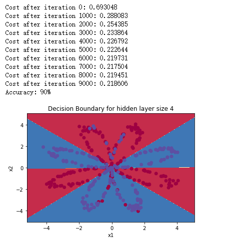
准确率高于logistic回归

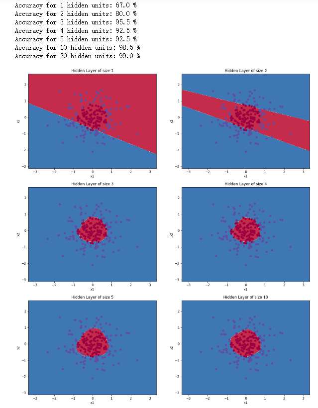
2.6 调整隐藏层大小

# This may take about 2 minutes to run

plt.figure(figsize=(16, 32))
hidden_layer_sizes = [1, 2, 3, 4, 5, 10, 20]
for i, n_h in enumerate(hidden_layer_sizes):
    plt.subplot(5, 2, i+1)
    plt.title('Hidden Layer of size %d' % n_h)
    parameters = nn_model(X, Y, n_h, num_iterations = 5000)
    plot_decision_boundary(lambda x: predict(parameters, x.T), X, Y)
    predictions = predict(parameters, X)
    accuracy = float((np.dot(Y,predictions.T) + np.dot(1-Y,1-predictions.T))/float(Y.size)*100)
    print ("Accuracy for {} hidden units: {} %".format(n_h, accuracy))

得到如下运行结果：

[外链图片转存失败,源站可能有防盗链机制,建议将图片保存下来直接上传(img-hN8BWS2u-1659012992274)(C:\Users\Jack London\AppData\Roaming\Typora\typora-user-images\image-20220727161738023.png)]

说明：

• 较大的模型能够更好地你和训练集
• 使用正则化可以防止过度拟合

2.7 使用其他数据集

# Datasets
noisy_circles, noisy_moons, blobs, gaussian_quantiles, no_structure = load_extra_datasets()

datasets = {"noisy_circles": noisy_circles,
            "noisy_moons": noisy_moons,
            "blobs": blobs,
            "gaussian_quantiles": gaussian_quantiles}

### START CODE HERE ### (choose your dataset)
dataset = "gaussian_quantiles"
### END CODE HERE ###

X, Y = datasets[dataset]
X, Y = X.T, Y.reshape(1, Y.shape[0])

# make blobs binary
if dataset == "blobs":
    Y = Y%2

# Visualize the data
plt.scatter(X[0, :], X[1, :], c=Y.reshape(X[0,:].shape), s=40, cmap=plt.cm.Spectral);

重新运行后得到如下结果：