


L2 改善深层神经网络
2 优化算法
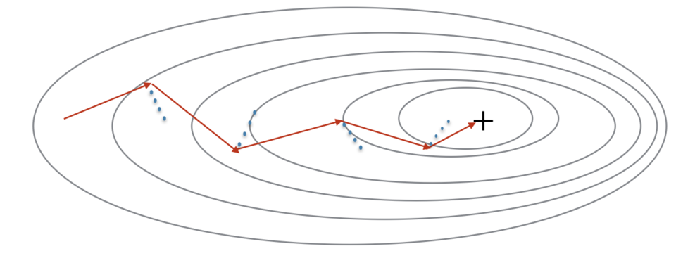
梯度下降法就好像是在损失函数 J J J上下坡
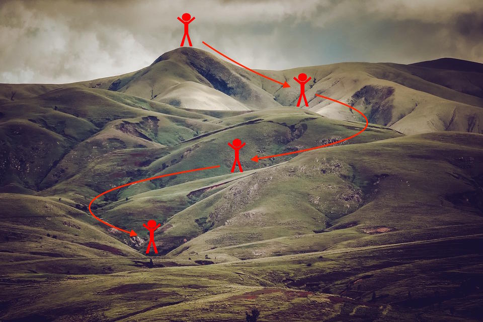
在训练的每个步骤中按照一定的方向更新参数,以尝试到达最低点
0 准备工作
首先引入所需的包
import numpy as np
import matplotlib.pyplot as plt
import scipy.io
import math
import sklearn
import sklearn.datasets

from opt_utils import load_params_and_grads, initialize_parameters, forward_propagation, backward_propagation
from opt_utils import compute_cost, predict, predict_dec, plot_decision_boundary, load_dataset
from testCases import *

%matplotlib inline
plt.rcParams['figure.figsize'] = (7.0, 4.0) # set default size of plots
plt.rcParams['image.interpolation'] = 'nearest'
plt.rcParams['image.cmap'] = 'gray'
1 梯度下降
热身练习:实现梯度下降更新方法
说明:梯度下降规则如下
W
[
l
]
=
W
[
l
]
−
α
d
W
[
l
]
b
[
l
]
=
b
[
l
]
−
α
d
b
[
l
]
W^{[l]} = W^{[l]}-\alpha dW^{[l]}\\ b^{[l]} = b^{[l]}-\alpha db^{[l]}
W[l]=W[l]−αdW[l]b[l]=b[l]−αdb[l]
其中l表示第l层,α是学习率
# GRADED FUNCTION: update_parameters_with_gd

def update_parameters_with_gd(parameters, grads, learning_rate):
    """
    Update parameters using one step of gradient descent

    Arguments:
    parameters -- python dictionary containing your parameters to be updated:
                    parameters['W' + str(l)] = Wl
                    parameters['b' + str(l)] = bl
    grads -- python dictionary containing your gradients to update each parameters:
                    grads['dW' + str(l)] = dWl
                    grads['db' + str(l)] = dbl
    learning_rate -- the learning rate, scalar.

    Returns:
    parameters -- python dictionary containing your updated parameters
    """

    L = len(parameters) // 2 # number of layers in the neural networks

    # Update rule for each parameter
    for l in range(L):
        parameters["W" + str(l+1)] = parameters["W" + str(l+1)] - learning_rate*grads["dW" + str(l+1)]
        parameters["b" + str(l+1)] = parameters["b" + str(l+1)] -learning_rate*grads["db" + str(l+1)]

    return parameters
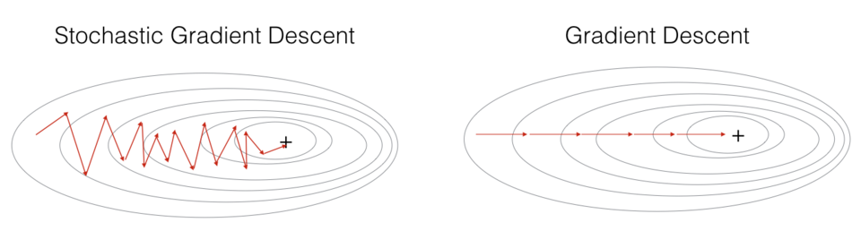
随机梯度下降SGD是基本梯度下降的一个变体
-
训练集大的时候可以更新更快
-
参数会向最小值摆动而不是平稳收敛,如下图所示:
-
实现SGD总共需要3个for循环
- 迭代次数
- m个训练数据
- 各层上的参数遍历
-
SGD相比mini-batch梯度下降
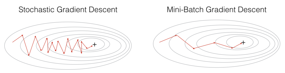
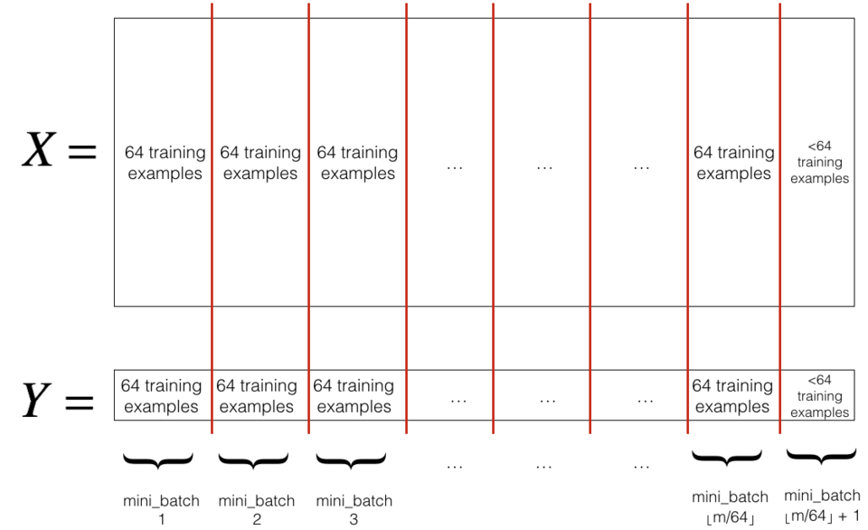
2 Mini-Batch梯度下降
在数据集中构建mini-batch:
-
Shuffle:打乱训练集
-
Partition:分割数据集
在python导入包中已经实现了shuffle部分
下面实现分割
# GRADED FUNCTION: random_mini_batches

def random_mini_batches(X, Y, mini_batch_size = 64, seed = 0):
    """
    Creates a list of random minibatches from (X, Y)

    Arguments:
    X -- input data, of shape (input size, number of examples)
    Y -- true "label" vector (1 for blue dot / 0 for red dot), of shape (1, number of examples)
    mini_batch_size -- size of the mini-batches, integer

    Returns:
    mini_batches -- list of synchronous (mini_batch_X, mini_batch_Y)
    """

    np.random.seed(seed)            # To make your "random" minibatches the same as ours
    m = X.shape[1]                  # number of training examples
    mini_batches = []

    # Step 1: Shuffle (X, Y)
    permutation = list(np.random.permutation(m))
    shuffled_X = X[:, permutation]
    shuffled_Y = Y[:, permutation].reshape((1,m))

    # Step 2: Partition (shuffled_X, shuffled_Y). Minus the end case.
    num_complete_minibatches = math.floor(m/mini_batch_size) # number of mini batches of size mini_batch_size in your partitionning
    for k in range(0, num_complete_minibatches):

        mini_batch_X = shuffled_X[:, k * mini_batch_size : (k+1) * mini_batch_size]
        mini_batch_Y = shuffled_Y[:, k * mini_batch_size : (k+1) * mini_batch_size]

        mini_batch = (mini_batch_X, mini_batch_Y)
        mini_batches.append(mini_batch)

    # Handling the end case (last mini-batch < mini_batch_size)
    if m % mini_batch_size != 0:

        mini_batch_X = shuffled_X[:, num_complete_minibatches * mini_batch_size : m]
        mini_batch_Y = shuffled_Y[:, num_complete_minibatches * mini_batch_size : m]

        mini_batch = (mini_batch_X, mini_batch_Y)
        mini_batches.append(mini_batch)

    return mini_batches
- 通常选择2的幂次作为最小批量大小
3 Momentum
mini-batch梯度下降在看到示例子集后才进行参数更新,更新方向有一定差异
使用momentum可以减少这些震荡,如下图所示:
momentum考虑了过去的梯度,用来进行平滑更新
将先前的梯度方向储存在变量 v v v中,可以看作是下坡滚动的球的速度
练习:初始化速度
# GRADED FUNCTION: initialize_velocity

def initialize_velocity(parameters):
    """
    Initializes the velocity as a python dictionary with:
                - keys: "dW1", "db1", ..., "dWL", "dbL"
                - values: numpy arrays of zeros of the same shape as the corresponding gradients/parameters.
    Arguments:
    parameters -- python dictionary containing your parameters.
                    parameters['W' + str(l)] = Wl
                    parameters['b' + str(l)] = bl

    Returns:
    v -- python dictionary containing the current velocity.
                    v['dW' + str(l)] = velocity of dWl
                    v['db' + str(l)] = velocity of dbl
    """

    L = len(parameters) // 2 # number of layers in the neural networks
    v = {}

    # Initialize velocity
    for l in range(L):
        v["dW" + str(l+1)] = np.zeros(parameters['W' + str(l+1)].shape)
        v["db" + str(l+1)] = np.zeros(parameters['b' + str(l+1)].shape)

    return v
练习:实现带momentum的参数更新
说明:更新规则为:
{
v
d
b
[
l
]
=
β
v
d
b
[
l
]
+
(
1
−
β
)
d
b
[
l
]
b
[
l
]
=
b
[
l
]
−
α
v
d
b
[
l
]
v
d
b
[
l
]
=
β
v
d
b
[
l
]
+
(
1
−
β
)
d
b
[
l
]
b
[
l
]
=
b
[
l
]
−
α
v
d
b
[
l
]
\begin{cases} v_{db^{[l]}} = \beta v_{db^{[l]}} + (1 - \beta) db^{[l]} \\ b^{[l]} = b^{[l]} - \alpha v_{db^{[l]}} \\\\ v_{db^{[l]}} = \beta v_{db^{[l]}} + (1 - \beta) db^{[l]} \\ b^{[l]} = b^{[l]} - \alpha v_{db^{[l]}} \end{cases}
⎩
⎨
⎧vdb[l]=βvdb[l]+(1−β)db[l]b[l]=b[l]−αvdb[l]vdb[l]=βvdb[l]+(1−β)db[l]b[l]=b[l]−αvdb[l]
# GRADED FUNCTION: update_parameters_with_momentum

def update_parameters_with_momentum(parameters, grads, v, beta, learning_rate):
    """
    Update parameters using Momentum

    Arguments:
    parameters -- python dictionary containing your parameters:
                    parameters['W' + str(l)] = Wl
                    parameters['b' + str(l)] = bl
    grads -- python dictionary containing your gradients for each parameters:
                    grads['dW' + str(l)] = dWl
                    grads['db' + str(l)] = dbl
    v -- python dictionary containing the current velocity:
                    v['dW' + str(l)] = ...
                    v['db' + str(l)] = ...
    beta -- the momentum hyperparameter, scalar
    learning_rate -- the learning rate, scalar

    Returns:
    parameters -- python dictionary containing your updated parameters
    v -- python dictionary containing your updated velocities
    """

    L = len(parameters) // 2 # number of layers in the neural networks

    # Momentum update for each parameter
    for l in range(L):

        # compute velocities
        v["dW" + str(l + 1)] = beta*v["dW" + str(l + 1)]+(1-beta)*grads['dW' + str(l+1)]
        v["db" + str(l + 1)] = beta*v["db" + str(l + 1)]+(1-beta)*grads['db' + str(l+1)]
        # update parameters
        parameters["W" + str(l + 1)] = parameters['W' + str(l+1)] - learning_rate*v["dW" + str(l + 1)]
        parameters["b" + str(l + 1)] = parameters['b' + str(l+1)] - learning_rate*v["db" + str(l + 1)]

    return parameters, v
说明:
- 速度采用0初始化
- 将会花费一些迭代来提高速度
- 如果β=0,则成为标准的梯度下降
- momentum将过去的梯度考虑在内,以平滑梯度进行下降
- 可以应用于批量梯度下降、mini-batch梯度下降或者SGD
如何选择β:
- β越大,更新越平滑
- 常用范围是[0.8, 0.999],默认0.9
4 Adam
Adam是训练神经网络最有效的优化算法之一,结合了RMSProp和Momentum的优点
Adam原理:
- 计算过去梯度的指数加权平均值
- 计算过去梯度的平方的指数加权平均值
- 组合“1”和“2”的信息,在一个方向上更新参数
练习:初始化跟踪过去信息的Adam变量 v , s v,s v,s
# GRADED FUNCTION: initialize_adam

def initialize_adam(parameters) :
    """
    Initializes v and s as two python dictionaries with:
                - keys: "dW1", "db1", ..., "dWL", "dbL"
                - values: numpy arrays of zeros of the same shape as the corresponding gradients/parameters.

    Arguments:
    parameters -- python dictionary containing your parameters.
                    parameters["W" + str(l)] = Wl
                    parameters["b" + str(l)] = bl

    Returns:
    v -- python dictionary that will contain the exponentially weighted average of the gradient.
                    v["dW" + str(l)] = ...
                    v["db" + str(l)] = ...
    s -- python dictionary that will contain the exponentially weighted average of the squared gradient.
                    s["dW" + str(l)] = ...
                    s["db" + str(l)] = ...

    """

    L = len(parameters) // 2 # number of layers in the neural networks
    v = {}
    s = {}

    # Initialize v, s. Input: "parameters". Outputs: "v, s".
    for l in range(L):
        v["dW" + str(l + 1)] = np.zeros(parameters["W" + str(l+1)].shape)
        v["db" + str(l + 1)] = np.zeros(parameters["b" + str(l+1)].shape)
        s["dW" + str(l + 1)] = np.zeros(parameters["W" + str(l+1)].shape)
        s["db" + str(l + 1)] = np.zeros(parameters["b" + str(l+1)].shape)

    return v, s
练习:用Adam实现参数更新
更新规则如下:
{
v
W
[
l
]
=
β
1
v
W
[
l
]
+
(
1
−
β
1
)
∂
J
∂
W
[
l
]
v
W
[
l
]
c
o
r
r
e
c
t
e
d
=
v
W
[
l
]
1
−
(
β
1
)
t
s
W
[
l
]
=
β
2
s
W
[
l
]
+
(
1
−
β
2
)
(
∂
J
∂
W
[
l
]
)
2
s
W
[
l
]
c
o
r
r
e
c
t
e
d
=
s
W
[
l
]
1
−
(
β
2
)
t
W
[
l
]
=
W
[
l
]
−
α
v
W
[
l
]
c
o
r
r
e
c
t
e
d
s
W
[
l
]
c
o
r
r
e
c
t
e
d
+
ε
\begin{cases} v_{W^{[l]}} = \beta_1 v_{W^{[l]}} + (1 - \beta_1) \frac{\partial J }{ \partial W^{[l]} } \\ v^{corrected}_{W^{[l]}} = \frac{v_{W^{[l]}}}{1 - (\beta_1)^t} \\ s_{W^{[l]}} = \beta_2 s_{W^{[l]}} + (1 - \beta_2) (\frac{\partial J }{\partial W^{[l]} })^2 \\ s^{corrected}_{W^{[l]}} = \frac{s_{W^{[l]}}}{1 - (\beta_2)^t} \\ W^{[l]} = W^{[l]} - \alpha \frac{v^{corrected}_{W^{[l]}}}{\sqrt{s^{corrected}_{W^{[l]}}}+\varepsilon} \end{cases}
⎩
⎨
⎧vW[l]=β1vW[l]+(1−β1)∂W[l]∂JvW[l]corrected=1−(β1)tvW[l]sW[l]=β2sW[l]+(1−β2)(∂W[l]∂J)2sW[l]corrected=1−(β2)tsW[l]W[l]=W[l]−αsW[l]corrected+εvW[l]corrected
注意:迭代器 l 在 for 循环中从0开始,而第一个参数是W[1]和b[1]。编码时需要将l转换为 l+1
# GRADED FUNCTION: update_parameters_with_adam

def update_parameters_with_adam(parameters, grads, v, s, t, learning_rate = 0.01,
                                beta1 = 0.9, beta2 = 0.999,  epsilon = 1e-8):
    """
    Update parameters using Adam

    Arguments:
    parameters -- python dictionary containing your parameters:
                    parameters['W' + str(l)] = Wl
                    parameters['b' + str(l)] = bl
    grads -- python dictionary containing your gradients for each parameters:
                    grads['dW' + str(l)] = dWl
                    grads['db' + str(l)] = dbl
    v -- Adam variable, moving average of the first gradient, python dictionary
    s -- Adam variable, moving average of the squared gradient, python dictionary
    learning_rate -- the learning rate, scalar.
    beta1 -- Exponential decay hyperparameter for the first moment estimates
    beta2 -- Exponential decay hyperparameter for the second moment estimates
    epsilon -- hyperparameter preventing division by zero in Adam updates

    Returns:
    parameters -- python dictionary containing your updated parameters
    v -- Adam variable, moving average of the first gradient, python dictionary
    s -- Adam variable, moving average of the squared gradient, python dictionary
    """

    L = len(parameters) // 2                 # number of layers in the neural networks
    v_corrected = {}                         # Initializing first moment estimate, python dictionary
    s_corrected = {}                         # Initializing second moment estimate, python dictionary

    # Perform Adam update on all parameters
    for l in range(L):
        # Moving average of the gradients. Inputs: "v, grads, beta1". Output: "v".
        v["dW" + str(l + 1)] = beta1*v["dW" + str(l + 1)] +(1-beta1)*grads['dW' + str(l+1)]
        v["db" + str(l + 1)] = beta1*v["db" + str(l + 1)] +(1-beta1)*grads['db' + str(l+1)]

        # Compute bias-corrected first moment estimate. Inputs: "v, beta1, t". Output: "v_corrected".
        v_corrected["dW" + str(l + 1)] = v["dW" + str(l + 1)]/(1-(beta1)**t)
        v_corrected["db" + str(l + 1)] = v["db" + str(l + 1)]/(1-(beta1)**t)

        # Moving average of the squared gradients. Inputs: "s, grads, beta2". Output: "s".
        s["dW" + str(l + 1)] =beta2*s["dW" + str(l + 1)] + (1-beta2)*(grads['dW' + str(l+1)]**2)
        s["db" + str(l + 1)] = beta2*s["db" + str(l + 1)] + (1-beta2)*(grads['db' + str(l+1)]**2)

        # Compute bias-corrected second raw moment estimate. Inputs: "s, beta2, t". Output: "s_corrected".
        s_corrected["dW" + str(l + 1)] =s["dW" + str(l + 1)]/(1-(beta2)**t)
        s_corrected["db" + str(l + 1)] = s["db" + str(l + 1)]/(1-(beta2)**t)

        # Update parameters. Inputs: "parameters, learning_rate, v_corrected, s_corrected, epsilon". Output: "parameters".
        parameters["W" + str(l + 1)] = parameters["W" + str(l + 1)]-learning_rate*(v_corrected["dW" + str(l + 1)]/np.sqrt( s_corrected["dW" + str(l + 1)]+epsilon))
        parameters["b" + str(l + 1)] = parameters["b" + str(l + 1)]-learning_rate*(v_corrected["db" + str(l + 1)]/np.sqrt( s_corrected["db" + str(l + 1)]+epsilon))

    return parameters, v, s
5 不同优化算法的模型
加载数据库
train_X, train_Y = load_dataset()
已经实现了一个三层的神经网络,将使用以下方法进行训练:
- mini-batch gradient descent
- mini-batch Momentum
- mini-batch Adam
神经网络代码如下所示:
def model(X, Y, layers_dims, optimizer, learning_rate = 0.0007, mini_batch_size = 64, beta = 0.9,
          beta1 = 0.9, beta2 = 0.999,  epsilon = 1e-8, num_epochs = 10000, print_cost = True):
    """
    3-layer neural network model which can be run in different optimizer modes.

    Arguments:
    X -- input data, of shape (2, number of examples)
    Y -- true "label" vector (1 for blue dot / 0 for red dot), of shape (1, number of examples)
    layers_dims -- python list, containing the size of each layer
    learning_rate -- the learning rate, scalar.
    mini_batch_size -- the size of a mini batch
    beta -- Momentum hyperparameter
    beta1 -- Exponential decay hyperparameter for the past gradients estimates
    beta2 -- Exponential decay hyperparameter for the past squared gradients estimates
    epsilon -- hyperparameter preventing division by zero in Adam updates
    num_epochs -- number of epochs
    print_cost -- True to print the cost every 1000 epochs

    Returns:
    parameters -- python dictionary containing your updated parameters
    """

    L = len(layers_dims)             # number of layers in the neural networks
    costs = []                       # to keep track of the cost
    t = 0                            # initializing the counter required for Adam update
    seed = 10                        # For grading purposes, so that your "random" minibatches are the same as ours

    # Initialize parameters
    parameters = initialize_parameters(layers_dims)

    # Initialize the optimizer
    if optimizer == "gd":
        pass # no initialization required for gradient descent
    elif optimizer == "momentum":
        v = initialize_velocity(parameters)
    elif optimizer == "adam":
        v, s = initialize_adam(parameters)

    # Optimization loop
    for i in range(num_epochs):

        # Define the random minibatches. We increment the seed to reshuffle differently the dataset after each epoch
        seed = seed + 1
        minibatches = random_mini_batches(X, Y, mini_batch_size, seed)

        for minibatch in minibatches:

            # Select a minibatch
            (minibatch_X, minibatch_Y) = minibatch

            # Forward propagation
            a3, caches = forward_propagation(minibatch_X, parameters)

            # Compute cost
            cost = compute_cost(a3, minibatch_Y)

            # Backward propagation
            grads = backward_propagation(minibatch_X, minibatch_Y, caches)

            # Update parameters
            if optimizer == "gd":
                parameters = update_parameters_with_gd(parameters, grads, learning_rate)
            elif optimizer == "momentum":
                parameters, v = update_parameters_with_momentum(parameters, grads, v, beta, learning_rate)
            elif optimizer == "adam":
                t = t + 1 # Adam counter
                parameters, v, s = update_parameters_with_adam(parameters, grads, v, s, t, learning_rate, beta1, beta2,  epsilon)

        # Print the cost every 1000 epoch
        if print_cost and i % 1000 == 0:
            print ("Cost after epoch %i: %f" %(i, cost))
        if print_cost and i % 100 == 0:
            costs.append(cost)

    # plot the cost
    plt.plot(costs)
    plt.ylabel('cost')
    plt.xlabel('epochs (per 100)')
    plt.title("Learning rate = " + str(learning_rate))
    plt.show()

    return parameters
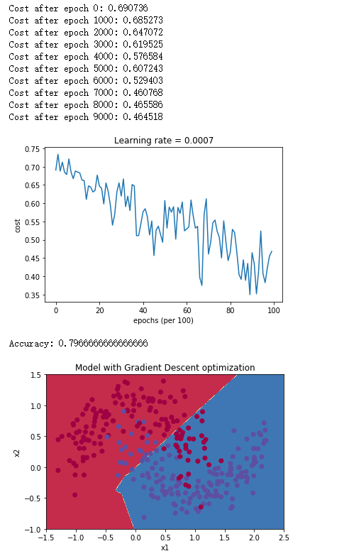
5.1 mini-batch梯度下降
使用如下代码进行测试:
# train 3-layer model
layers_dims = [train_X.shape[0], 5, 2, 1]
parameters = model(train_X, train_Y, layers_dims, optimizer = "gd")

# Predict
predictions = predict(train_X, train_Y, parameters)

# Plot decision boundary
plt.title("Model with Gradient Descent optimization")
axes = plt.gca()
axes.set_xlim([-1.5,2.5])
axes.set_ylim([-1,1.5])
plot_decision_boundary(lambda x: predict_dec(parameters, x.T), train_X, train_Y)
得到如下结果:
注意此处绘图有bug,需要将opt_utils.py第232行修改为如下形式
plt.scatter(X[0, :], X[1, :], c=y.ravel(), cmap=plt.cm.Spectral)
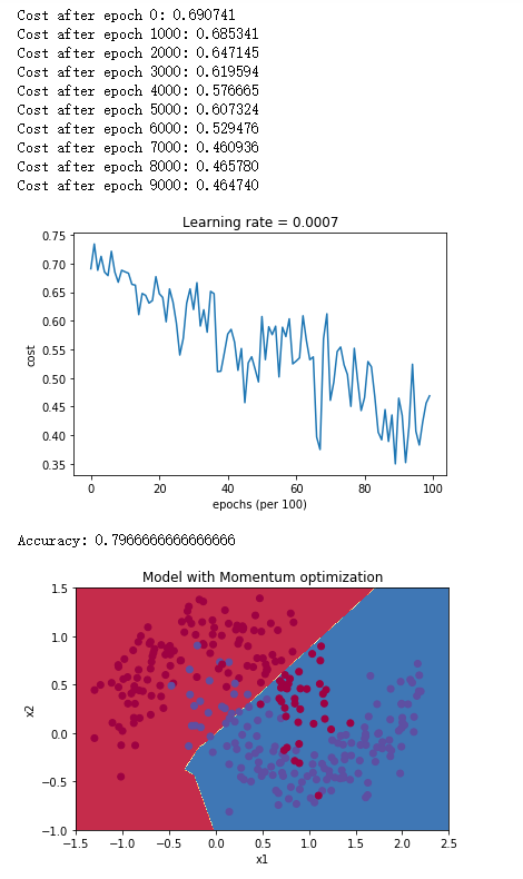
5.2 Momentum的mini-batch梯度下降
使用如下代码进行测试:
# train 3-layer model
layers_dims = [train_X.shape[0], 5, 2, 1]
parameters = model(train_X, train_Y, layers_dims, beta = 0.9, optimizer = "momentum")

# Predict
predictions = predict(train_X, train_Y, parameters)

# Plot decision boundary
plt.title("Model with Momentum optimization")
axes = plt.gca()
axes.set_xlim([-1.5,2.5])
axes.set_ylim([-1,1.5])
plot_decision_boundary(lambda x: predict_dec(parameters, x.T), train_X, train_Y)
得到如下结果:
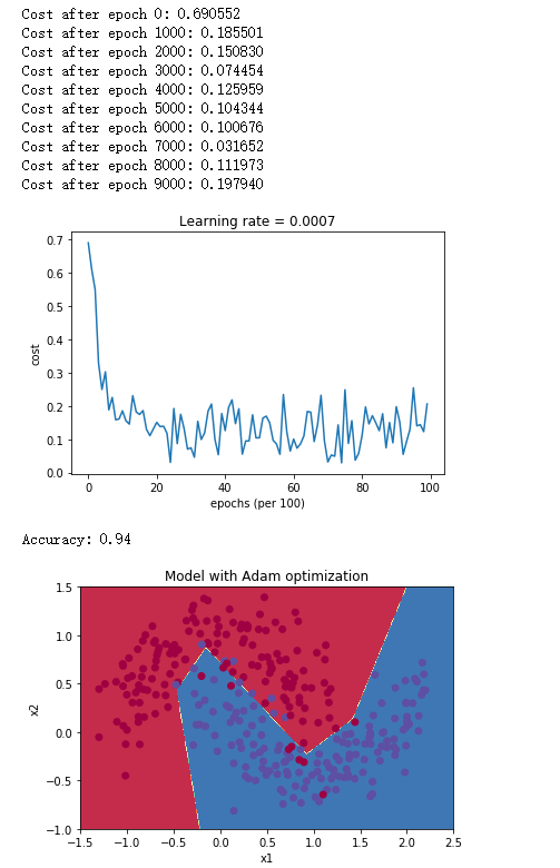
5.3 Adam的mini-batch梯度下降
使用如下代码进行测试:
# train 3-layer model
layers_dims = [train_X.shape[0], 5, 2, 1]
parameters = model(train_X, train_Y, layers_dims, optimizer = "adam")

# Predict
predictions = predict(train_X, train_Y, parameters)

# Plot decision boundary
plt.title("Model with Adam optimization")
axes = plt.gca()
axes.set_xlim([-1.5,2.5])
axes.set_ylim([-1,1.5])
plot_decision_boundary(lambda x: predict_dec(parameters, x.T), train_X, train_Y)
得到如下结果:
5.4 总结
| 优化方法 | 准确度 | 模型损失 |
|---|---|---|
| Gradient descent | 79.70% | 振荡 |
| Momentum | 79.70% | 振荡 |
| Adam | 94% | 更光滑 |
可见:
- Momentum会有一定帮助,但是由于学习率低、数据集简单,影响很小
- Adam明显优于mini-batch梯度下降和Momentum梯度下降
Adam优势包括:
- 相对较低的内存要求
- 但是高于梯度下降和Momentum的梯度湘江
- 即使很少超参数,也能较好进行
Adam论文:https://arxiv.org/pdf/1412.6980.pdf


 536
536


 被折叠的 条评论
为什么被折叠?
被折叠的 条评论
为什么被折叠?
 到【灌水乐园】发言


