深度学习用于疾病预后-第二课第二周大作业-练习基于树和随机森林构建风险模型（强推，干货多）

使用基于树的模型的风险模型

作业地址

github -->  bharathikannann/AI-for-Medicine-Specialization-deeplearning.ai

在此作业中，您将通过预测来自 NHANES I 流行病学数据集的个人 10 年死亡风险来获得基于树的模型的经验（有关此数据集的详细描述，您可以查看 CDC Website）。

这是一项具有挑战性的任务，也是我们本周学习的机器学习方法的一个很好的测试平台。

在完成作业时，您将了解：

• 处理缺失数据
  • 完成案例分析。
  • 插补
• 决策树
  • 评估。
  • 正则化。
• 随机森林
  • 超参数调整。

1 导入包

• shap 是一个解释机器学习模型所做预测的库。
• sklearn 是最受欢迎的机器学习库之一。
• itertools允许我们方便地操作可迭代对象，例如列表。
• pydotplus与 IPython.display.Image 一起使用以可视化图形结构，例如决策树。
• numpy是 Python 科学计算的基础包。
• pandas是我们将用来操纵数据的东西。
• seaborn是一个绘图库，它有一些方便的函数来可视化丢失的数据。
• matplotlib是一个绘图库。

import shap
import sklearn
import itertools
import pydotplus
import numpy as np
import pandas as pd
import seaborn as sns
import matplotlib.pyplot as plt

from IPython.display import Image 

from sklearn.tree import export_graphviz
from sklearn.externals.six import StringIO
from sklearn.tree import DecisionTreeClassifier
from sklearn.ensemble import RandomForestClassifier
from sklearn.model_selection import train_test_split
from sklearn.experimental import enable_iterative_imputer
from sklearn.impute import IterativeImputer, SimpleImputer

# We'll also import some helper functions that will be useful later on.
from util import load_data, cindex

注意：如果这一步遇到错误如下：

ModuleNotFoundError: No module named 'sklearn.externals.six'

把这个模块改为

from six import StringIO  
# from sklearn.externals.six import StringIO 
# sklearn.externals.six 模块在 scikit-learn 0.23 及以后的版本已经被删除。

2 加载数据

运行下一个单元格以加载到 NHANES I 流行病学数据集中。该数据集包含医院患者的各种特征及其结果，即他们是否在 10 年内死亡。

X_dev, X_test, y_dev, y_test = load_data(10)
X_train, X_val, y_train, y_val = train_test_split(X_dev, y_dev, test_size=0.25, random_state=10)

数据集已分为一个开发集（或dev），我们将使用它来开发我们的风险模型，以及一个测试集，我们将使用它来测试我们的模型。

我们进一步将开发集分成训练集和验证集，分别使用 75/25 分割来训练和调整我们的模型（请注意，我们设置了一个随机状态以使该分割可重复）。

3 探索数据

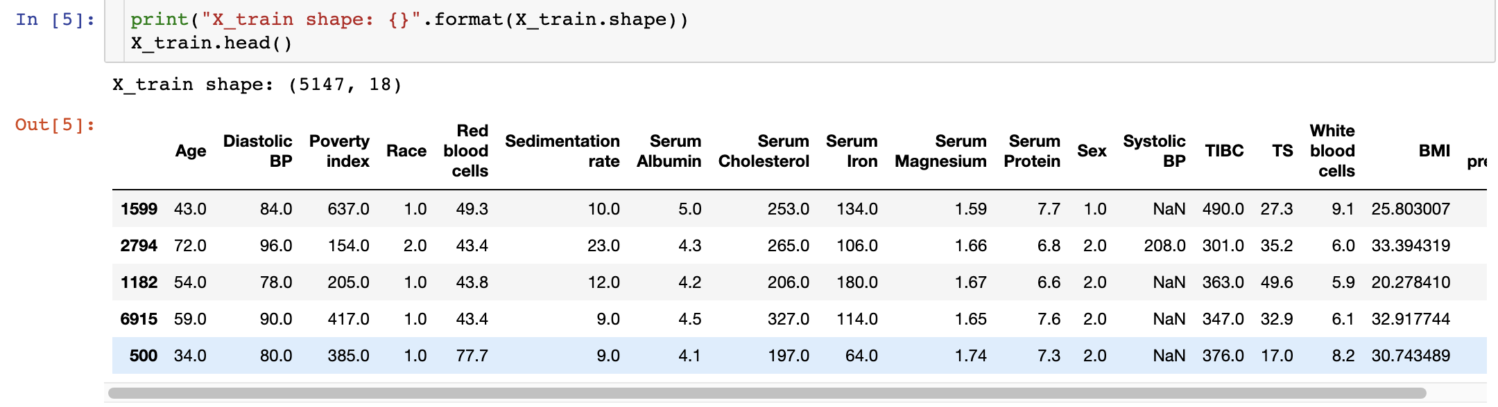
从图中可以看出，这个数据一共有5147个患者，每个患者有18个特征。

4 处理缺失数据

查看 X_train 中的数据，我们发现缺少一些数据：上图中的一些值被标记为NaN（“不是数字”）。

数据缺失是数据分析中常见的现象，可能由多种原因造成，如测量仪器故障、受访者不愿意或不能提供信息、数据收集过程中的错误等。

让我们检查丢失的数据模式。seaborn是一个替代品，matplotlib它有一些方便的数据分析绘图功能。我们可以使用它的heatmap功能轻松可视化丢失的数据模式。

sns.heatmap(X_train.isnull(), cbar=False)
plt.title("Training")
plt.show()

sns.heatmap(X_val.isnull(), cbar=False)
plt.title("Validation")
plt.show()

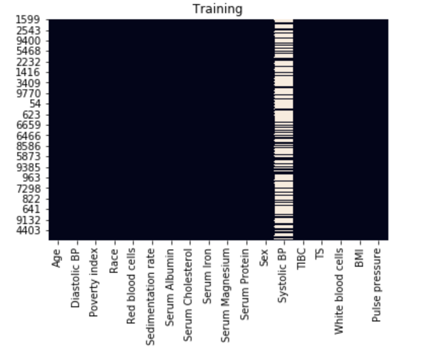
对于表示为一列的每个特征，存在的值显示为黑色，缺失值设置为浅色。
从该图中，我们可以看到收缩压 (Systolic BP) 缺少许多值。

在下面的单元格中，编写一个函数来计算具有缺失数据的个案分数。这将帮助我们决定将来如何处理这些缺失的数据。

# UNQ_C1 (UNIQUE CELL IDENTIFIER, DO NOT EDIT)
def fraction_rows_missing(df):
    '''
    Return percent of rows with any missing
    data in the dataframe. 
    
    Input:
        df (dataframe): a pandas dataframe with potentially missing data
    Output:
        frac_missing (float): fraction of rows with missing data
    '''
    ### START CODE HERE (REPLACE 'Pass' with your 'return' code) ###
    return np.sum(pd.DataFrame.any(df.isnull(),axis = 1)) / df.shape[0]  
    ### END CODE HERE ###

• pandas.DataFrame.isnull()方法在这种情况下很有用。
• 使用该pandas.DataFrame.any()方法并设置axis参数。
• 将包含缺失数据的总行数除以总行数。请记住，在 Python 中，True值等于 1。

df_test = pd.DataFrame({'a':[None, 1, 1, None], 'b':[1, None, 0, 1]})
print("Example dataframe:\n")
print(df_test)

print("\nComputed fraction missing: {}, expected: {}".format(fraction_rows_missing(df_test), 0.75))
print(f"Fraction of rows missing from X_train: {fraction_rows_missing(X_train):.3f}")
print(f"Fraction of rows missing from X_val: {fraction_rows_missing(X_val):.3f}")
print(f"Fraction of rows missing from X_test: {fraction_rows_missing(X_test):.3f}")

Computed fraction missing: 0.75, expected: 0.75
Fraction of rows missing from X_train: 0.699
Fraction of rows missing from X_val: 0.704
Fraction of rows missing from X_test: 0.000

我们看到我们的训练集和验证集有缺失值，但幸运的是我们的测试集有完整的案例。

作为第一步，我们将从完整的案例分析开始，删除所有包含任何缺失数据的行。运行以下单元格以从我们的训练和验证集中删除这些行。

X_train_dropped = X_train.dropna(axis='rows')
y_train_dropped = y_train.loc[X_train_dropped.index]
X_val_dropped = X_val.dropna(axis='rows')
y_val_dropped = y_val.loc[X_val_dropped.index]

5 决策树

刚刚学习了决策树，您选择使用决策树分类器。使用 scikit-learn 使用训练集为医院数据集构建决策树。

dt = DecisionTreeClassifier(max_depth=None, random_state=10)
dt.fit(X_train_dropped, y_train_dropped)

接下来我们将评估我们的模型。我们将使用 C-Index 进行评估。

记还记得第1周的第4课吗，c指数评估模型区分不同类别的能力，通过量化在考虑所有患者对(A, B)时，模型认为患者A的风险评分高于患者B，而在观察到的数据中，患者a实际死亡，而患者B实际存活。在我们的例子中，我们的模型是一个二元分类器，其中每个风险评分要么是1(模型预测患者会死亡)，要么是0(患者会活下来)。

更正式地说，将允许的患者对定义为结果不同的对，将一致的患者对定义为死亡患者具有更高风险评分的允许对（即我们的模型预测死亡患者为 1，存活患者为 0） , 并且作为风险评分相等的允许对联系在一起（即我们的模型预测两个患者为 1 或两个患者为 0），C 指数等于：
$$\text{C-Index}=\frac{\#\text{concordant pairs}+0.5\times \#\text{ties}}{\#\text{permissible pairs}}$$

注意：如果你忘记了C-Index的具体内容，查看第二课第一周第9-11节部分。
第二课第一周第9-11节 评估预后模型+作业解析

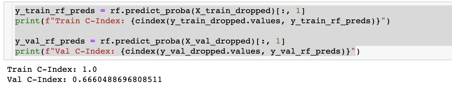
运行下一个单元格以计算训练集和验证集上的 C-Index（这次我们为您提供了一个实现）

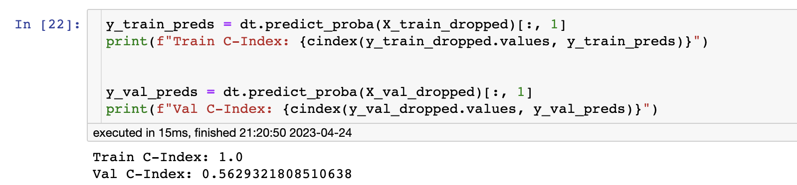
不幸的是，您的树似乎过度拟合：它非常适合训练数据，以至于不能很好地推广到其他样本，例如来自验证集的样本。

训练 C-index 为 1.0，因为在初始化时DecisionTreeClasifier，我们没有max_depth指定min_samples_split。因此，生成的决策树将尽可能地分裂，这几乎可以保证完全适合训练数据。

要处理这个问题，您可以更改我们树的一些超参数。

尝试找到一组提高对验证集的泛化能力的超参数，并重新计算 C-index。如果你做对了，你应该让验证集的 C-index 高于 0.6。

比如，尝试限制树的深度max_depth。

dt_hyperparams = {
    # set your own hyperparameters below, such as 'min_samples_split': 1

    ### START CODE HERE ###
    'max_depth' : 20,
    'min_samples_split' : 0.5
    
    ### END CODE HERE ###
}

# UNQ_C2 (UNIQUE CELL IDENTIFIER, DO NOT EDIT)
dt_reg = DecisionTreeClassifier(**dt_hyperparams, random_state=10)
dt_reg.fit(X_train_dropped, y_train_dropped)

y_train_preds = dt_reg.predict_proba(X_train_dropped)[:, 1]
y_val_preds = dt_reg.predict_proba(X_val_dropped)[:, 1]
print(f"Train C-Index: {cindex(y_train_dropped.values, y_train_preds)}")
print(f"Val C-Index (expected > 0.6): {cindex(y_val_dropped.values, y_val_preds)}")

Train C-Index: 0.6201372530835575
Val C-Index (expected > 0.6): 0.6116855053191489

如果使用较低的max_depth，则可以打印整个树。这允许易于解释。运行下一个单元格来打印树的分裂

dot_data = StringIO()
export_graphviz(dt_reg, feature_names=X_train_dropped.columns, out_file=dot_data,  
                filled=True, rounded=True, proportion=True, special_characters=True,
                impurity=False, class_names=['neg', 'pos'], precision=2)
graph = pydotplus.graph_from_dot_data(dot_data.getvalue())  
Image(graph.create_png())

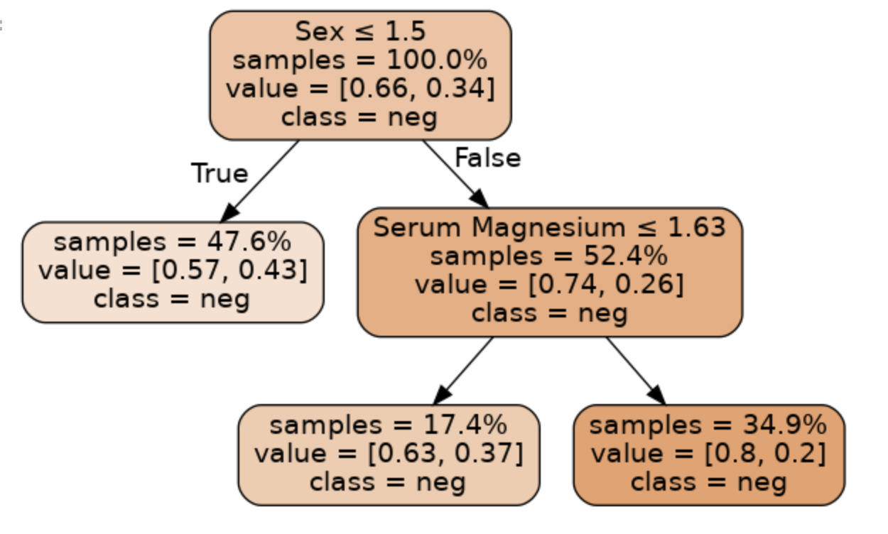
注意：我在最后一行代码报错了，没有画出决策树。没时间改bug, 继续往下学写了~~~

6 随机森林

无论你如何选择超参数，单个决策树都容易出现过拟合。要解决这个问题，您可以尝试随机森林，它结合来自许多不同树的预测来创建一个强大的分类器。

和以前一样，我们将使用 scikit-learn 为数据构建随机森林。我们将使用默认的超参数。

rf = RandomForestClassifier(n_estimators=100, random_state=10)
rf.fit(X_train_dropped, y_train_dropped)

使用默认超参数训练随机森林会产生比上一节中的单个决策树具有更好预测性能的模型，但该模型会过度拟合。

因此，我们需要调整（或优化）超参数，以找到一个既具有良好预测性能又能最大限度地减少过度拟合的模型。

我们选择调整的超参数将是：

• n_estimators：森林中使用的树木数量。
• max_depth：每棵树的最大深度。
• min_samples_leaf:叶子中样本的最小数量 (if int) 或比例(if float)。
  我们实施的调整超参数的方法称为网格搜索：
• 我们为每个目标超参数定义了一组可能的值。
• 针对每个可能的超参数组合训练和评估模型。
• 返回性能最佳的一组超参数。

下面的单元格实现了超参数网格搜索，使用 C-Index 来评估每个测试模型。

def holdout_grid_search(clf, X_train_hp, y_train_hp, X_val_hp, y_val_hp, hyperparams, fixed_hyperparams={}):
    '''
    Conduct hyperparameter grid search on hold out validation set. Use holdout validation.
    Hyperparameters are input as a dictionary mapping each hyperparameter name to the
    range of values they should iterate over. Use the cindex function as your evaluation
    function.

    Input:
        clf: sklearn classifier
        X_train_hp (dataframe): dataframe for training set input variables
        y_train_hp (dataframe): dataframe for training set targets
        X_val_hp (dataframe): dataframe for validation set input variables
        y_val_hp (dataframe): dataframe for validation set targets
        hyperparams (dict): hyperparameter dictionary mapping hyperparameter
                            names to range of values for grid search
        fixed_hyperparams (dict): dictionary of fixed hyperparameters that
                                  are not included in the grid search

    Output:
        best_estimator (sklearn classifier): fitted sklearn classifier with best performance on
                                             validation set
        best_hyperparams (dict): hyperparameter dictionary mapping hyperparameter
                                 names to values in best_estimator
    '''
    best_estimator = None
    best_hyperparams = {}
    
    # hold best running score
    best_score = 0.0

    # get list of param values
    lists = hyperparams.values()
    
    # get all param combinations
    param_combinations = list(itertools.product(*lists))
    total_param_combinations = len(param_combinations)

    # iterate through param combinations
    for i, params in enumerate(param_combinations, 1):
        # fill param dict with params
        param_dict = {}
        for param_index, param_name in enumerate(hyperparams):
            param_dict[param_name] = params[param_index]
            
        # create estimator with specified params
        estimator = clf(**param_dict, **fixed_hyperparams)

        # fit estimator
        estimator.fit(X_train_hp, y_train_hp)
        
        # get predictions on validation set
        preds = estimator.predict_proba(X_val_hp)
        
        # compute cindex for predictions
        estimator_score = cindex(y_val_hp, preds[:,1])

        print(f'[{i}/{total_param_combinations}] {param_dict}')
        print(f'Val C-Index: {estimator_score}\n')

        # if new high score, update high score, best estimator
        # and best params 
        if estimator_score >= best_score:
                best_score = estimator_score
                best_estimator = estimator
                best_hyperparams = param_dict

    # add fixed hyperparamters to best combination of variable hyperparameters
    best_hyperparams.update(fixed_hyperparams)
    
    return best_estimator, best_hyperparams

在下面的单元格中，定义要对其运行超参数网格搜索的值，然后运行该单元格以查找性能最佳的一组超参数。

您的目标是在训练集和验证集上获得高于0.6的C-Index。

• n_estimators：尝试大于 100 的值
• max_depth：尝试 1 到 100 范围内的值
• min_samples_leaf：尝试低于 .5 的浮点值和/或大于 2 的整数值

def random_forest_grid_search(X_train_dropped, y_train_dropped, X_val_dropped, y_val_dropped):

    # Define ranges for the chosen random forest hyperparameters 
    hyperparams = {
        
        ### START CODE HERE (REPLACE array values with your code) ###

        # how many trees should be in the forest (int)
        'n_estimators': [10],

        # the maximum depth of trees in the forest (int)
        
        'max_depth': [5],
        
        # the minimum number of samples in a leaf as a fraction
        # of the total number of samples in the training set
        # Can be int (in which case that is the minimum number)
        # or float (in which case the minimum is that fraction of the
        # number of training set samples)
        'min_samples_leaf': [1],

        ### END CODE HERE ###
    }

    
    fixed_hyperparams = {
        'random_state': 10,
    }
    
    rf = RandomForestClassifier

    best_rf, best_hyperparams = holdout_grid_search(rf, X_train_dropped, y_train_dropped,
                                                    X_val_dropped, y_val_dropped, hyperparams,
                                                    fixed_hyperparams)

    print(f"Best hyperparameters:\n{best_hyperparams}")

    
    y_train_best = best_rf.predict_proba(X_train_dropped)[:, 1]
    print(f"Train C-Index: {cindex(y_train_dropped, y_train_best)}")

    y_val_best = best_rf.predict_proba(X_val_dropped)[:, 1]
    print(f"Val C-Index: {cindex(y_val_dropped, y_val_best)}")
    
    # add fixed hyperparamters to best combination of variable hyperparameters
    best_hyperparams.update(fixed_hyperparams)
    
    return best_rf, best_hyperparams

best_rf, best_hyperparams = random_forest_grid_search(X_train_dropped, y_train_dropped, X_val_dropped, y_val_dropped)

结果：

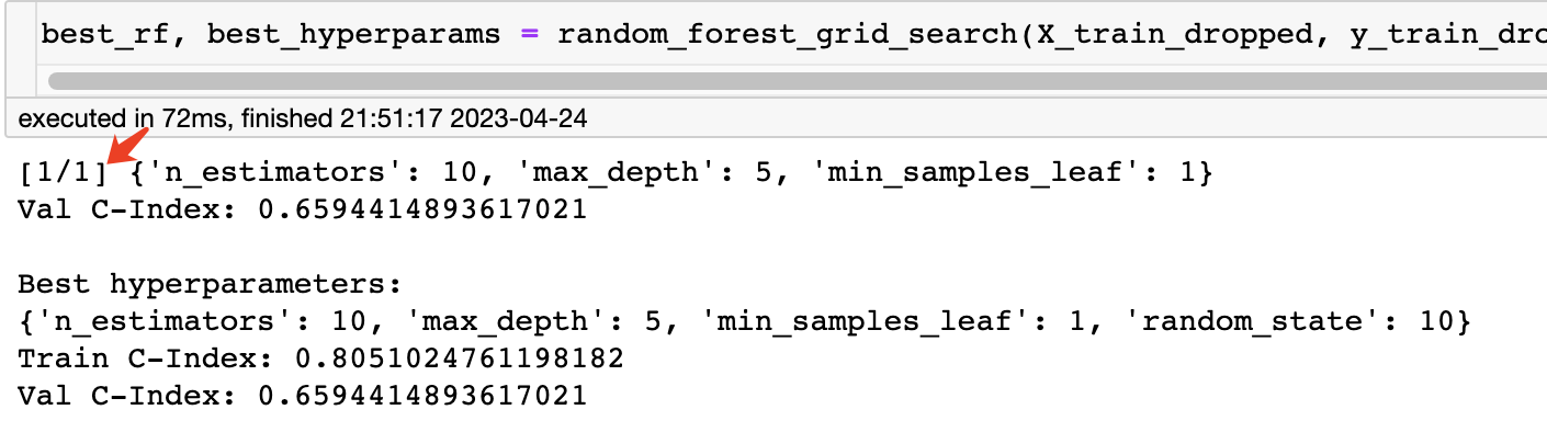
注意，在这里并没有真正用到网格搜索，因为只提供了一种情况。
我们修改这部分代码为：

hyperparams = {
        
        ### START CODE HERE (REPLACE array values with your code) ###

        # how many trees should be in the forest (int)
        'n_estimators': [10, 20, 30],

        # the maximum depth of trees in the forest (int)
        
        'max_depth': [5, 6],
        
        # the minimum number of samples in a leaf as a fraction
        # of the total number of samples in the training set
        # Can be int (in which case that is the minimum number)
        # or float (in which case the minimum is that fraction of the
        # number of training set samples)
        'min_samples_leaf': [1, 0.5],

        ### END CODE HERE ###
    }

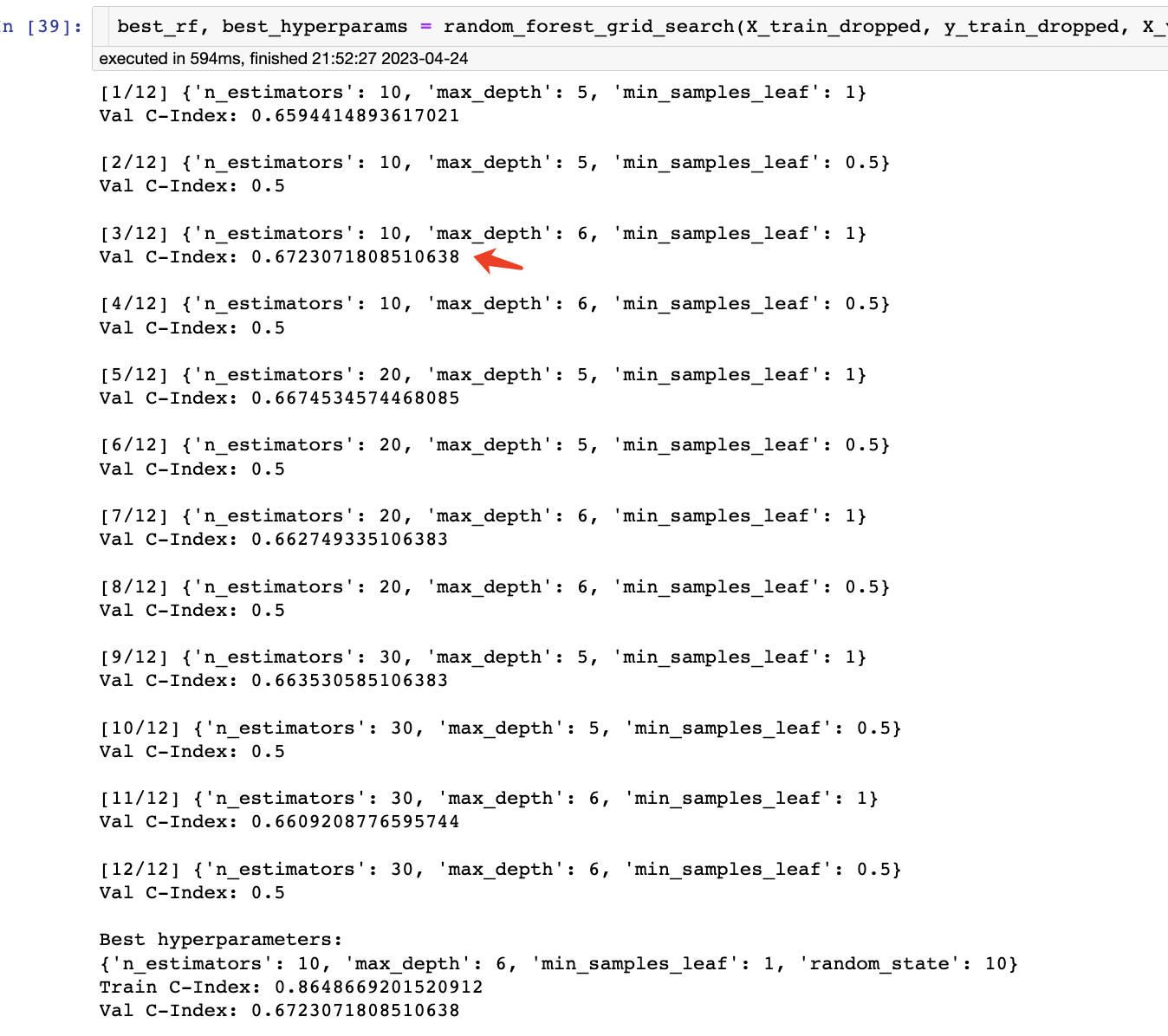
可以看到，一共有12种组合，并给出了最佳组合的超参数。

7 插值

现在，您已经根据我们的数据构建并优化了一个随机森林模型。但是，测试C-Index仍然有所下降。这可能是因为你丢掉了我们数据中超过一半的数据，因为收缩压的值缺失了。相反，我们可以尝试填充或输入这些值。

首先，让我们看看我们的数据是否是随机丢失的。让我们根据每个协变量(收缩压除外)绘制下降行的直方图，看看是否存在趋势。将这些与整个数据集中特征的直方图进行比较。试着看看其中一个协变量在两个子集中是否有显著不同的分布。

dropped_rows = X_train[X_train.isnull().any(axis=1)]

columns_except_Systolic_BP = [col for col in X_train.columns if col not in ['Systolic BP']]

for col in columns_except_Systolic_BP:
    sns.distplot(X_train.loc[:, col], norm_hist=True, kde=False, label='full data')
    sns.distplot(dropped_rows.loc[:, col], norm_hist=True, kde=False, label='without missing data')
    plt.legend()

    plt.show()

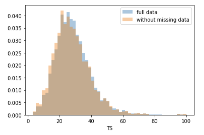
无论我们是否丢弃了缺少数据的行，大多数协变量的分布都是类似的。换句话说，数据的缺失与这些协变量无关。

如果所有协变量都是这样，那么数据就会被认为是完全随机缺失的（MCAR）。

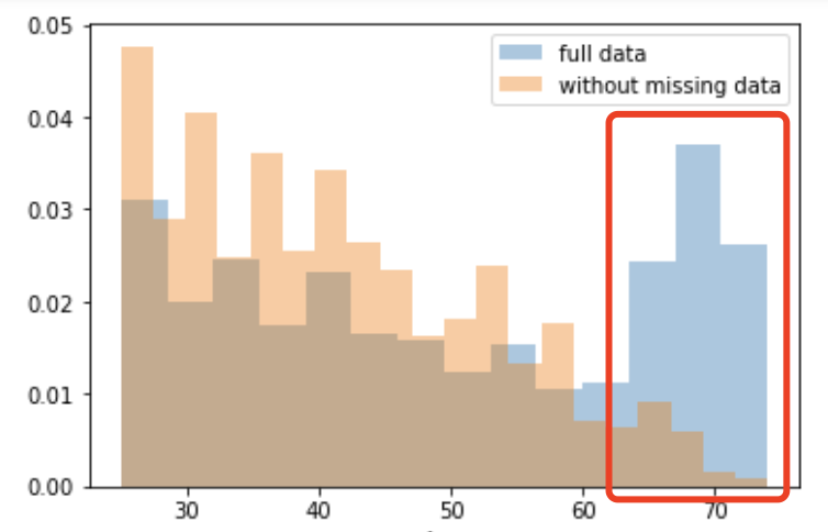
但当考虑年龄协变量时，我们发现65岁以上的患者往往会缺少更多的数据。原因可能是老年人测量血压的频率较低，以避免给他们带来额外的负担。

由于缺失与一个或多个协变量有关，因此缺失的数据被称为随机缺失（MAR）。

然而，根据我们掌握的信息，没有理由相信缺失数据的值，特别是缺失的收缩压的值，与患者的年龄有关。如果是这种情况，那么这些数据将被认为是非随机丢失的（MNAR）。

之前讲过插补常用两种方法，均值插补和回归插补，接下来就学习将理论转化为代码

均值插补

# Impute values using the mean
imputer = SimpleImputer(strategy='mean')
imputer.fit(X_train)
X_train_mean_imputed = pd.DataFrame(imputer.transform(X_train), columns=X_train.columns)

使用sklearn的SimpleImputer就可以完成插值啦

回归插补

接下来，我们将使用sklearn的IterativeImputter类应用另一种插补策略，称为多元特征插补。

使用该策略，对于每个缺失值的特征，训练回归模型以基于所有其他特征预测观测值，并使用该模型推断缺失值。由于在所有特征上的一次迭代可能不足以估算所有缺失的值，因此可以执行多次迭代

# Impute using regression on other covariates
imputer = IterativeImputer(random_state=0, sample_posterior=False, max_iter=3, min_value=0)
imputer.fit(X_train)
X_train_imputed = pd.DataFrame(imputer.transform(X_train), columns=X_train.columns)
X_val_imputed = pd.DataFrame(imputer.transform(X_val), columns=X_val.columns)

最后，我们比较一下不插值，均值插补，回归插补对结果的影响，这里选择了一个子集用来验证。

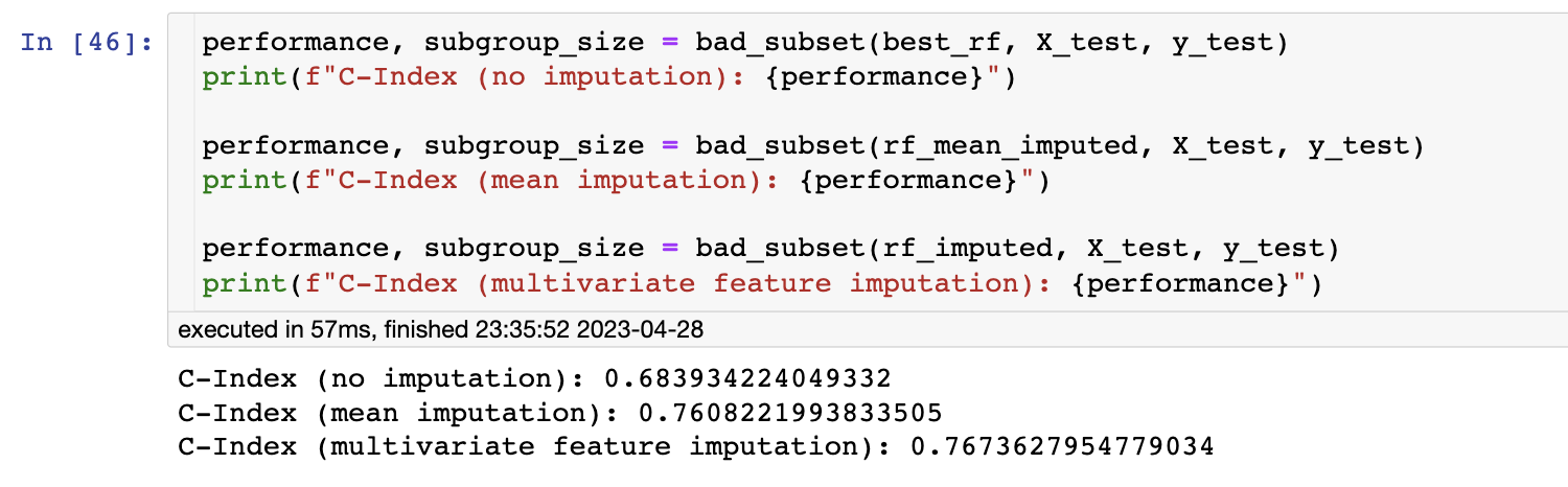
我们应该看到，完整的案例分析（即只对没有遗漏数据的观测结果进行分析）可以让我们的模型更好地泛化。记得检查你的缺失数据，判断它们是否随机缺失

可解释性

使用随机森林改善了结果，但我们已经失去了树木的一些自然可解释性。在本节中，我们将尝试使用稍微复杂一些的技术来解释这些预测。

您选择应用 SHAP (SHapley Additive exPlanations)，这是一种解释黑箱机器学习模型（即过于复杂而无法被人类理解的模型）所做预测的前沿方法。

给定由机器学习模型进行的预测，SHAP值通过量化每个特征对预测的附加重要性来解释预测。SHAP值源于合作博弈论，其中Shapley值用于量化每个玩家对游戏的贡献。

尽管计算一般黑盒模型的SHAP值在计算上很昂贵，但在树木和森林的情况下，存在一种快速多项式时间算法。有关更多详细信息，see the TreeShap paper.

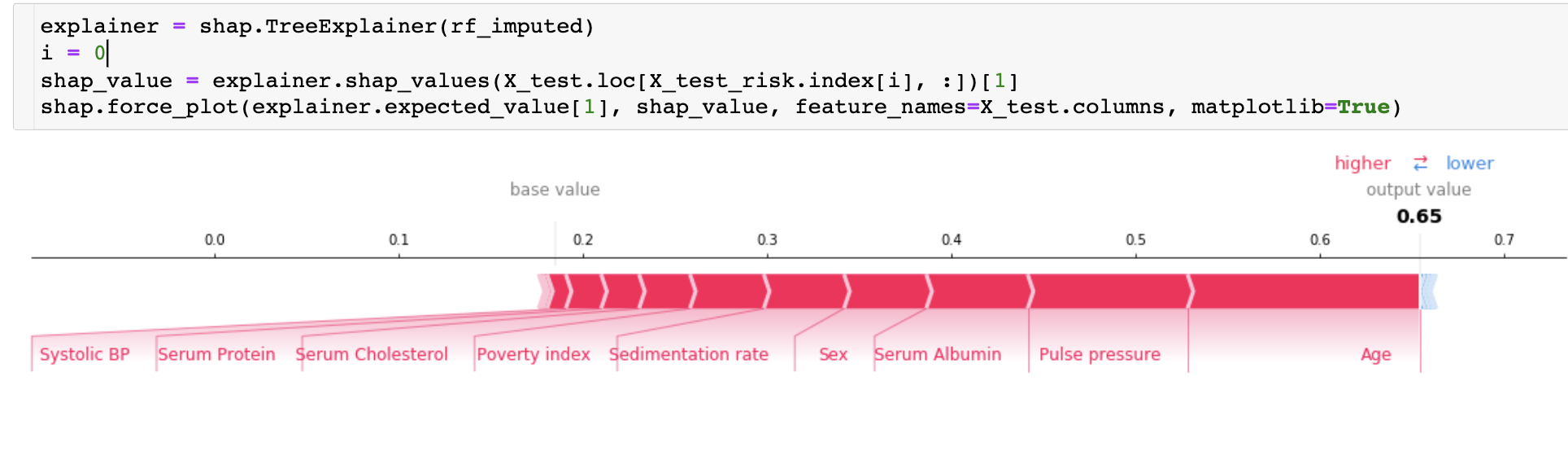
如何阅读此图表：

• 左侧的红色部分是将模型推向正方向的最终预测的特征（即，年龄越大，预测的风险越大）。
• 右侧的蓝色部分是将模型推向负方向的最终预测的特征（如果特征的增加导致风险降低，则将以蓝色显示）。
• 请注意，根据您为模型选择的超参数，图表的确切输出会有所不同。

我们还可以使用SHAP值来理解模型的总体输出。运行下一个单元格以初始化SHAP值（这可能需要几分钟时间）。

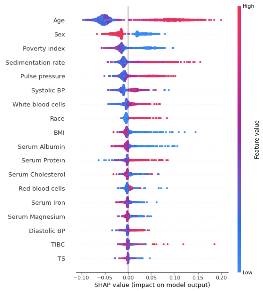
很明显，我们看到女性（性别=2.0，而男性的性别=1.0）的SHAP值为负，这意味着它降低了10年内死亡的风险。高年龄和高收缩压具有正的SHAP值，因此与死亡率增加有关。

您可以使用依赖关系图来查看要素是如何交互的。这些为每个数据点绘制给定特征的SHAP值，并使用另一个特征的值为点上色。这让我们开始解释主要功能的单个值的SHAP值的变化。

shap.dependence_plot('Age', shap_values, X_test, interaction_index='Sex')

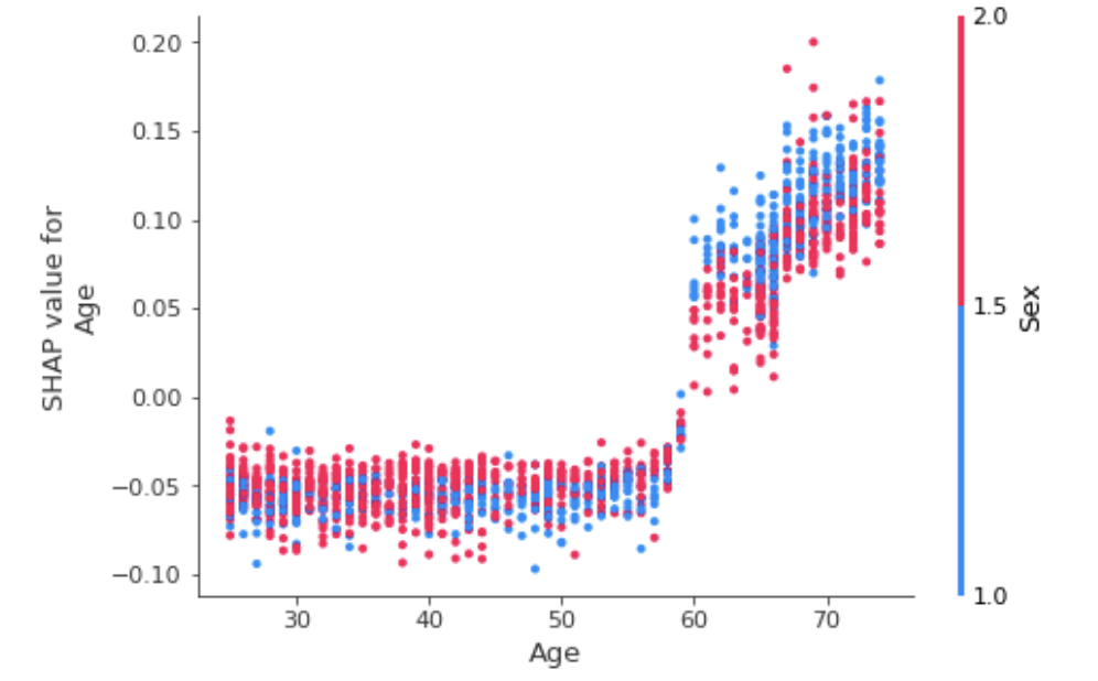
我们发现，虽然年龄＞60通常是不好的（SHAP值为正），但作为一名女性通常会减少年龄的影响。这是有道理的，因为我们知道女性通常比男性活得更长。

现在让我们看看贫困指数和年龄

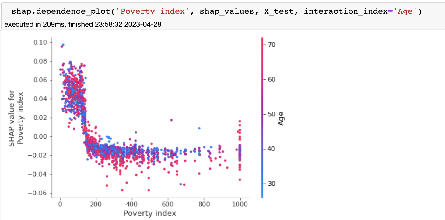
我们看到，贫困指数的影响迅速下降，对于高收入个体，年龄开始解释贫困指数影响的很大变化。

当然，你也可以观察其他的特征对。

本节代码很多，涉及的概念很多。代码解读只是其中的一部分，深刻理解还需要自己亲自跑一遍。

文章持续更新，可以关注微信公众号【医学图像人工智能实战营】获取最新动态，一个关注于医学图像处理领域前沿科技的公众号。坚持已实践为主，手把手带你做项目，打比赛，写论文。凡原创文章皆提供理论讲解，实验代码，实验数据。只有实践才能成长的更快，关注我们，一起学习进步~

我是Tina, 我们下篇博客见~

白天工作晚上写文，呕心沥血

觉得写的不错的话最后，求点赞，评论，收藏。或者一键三连