零基础入门深度学习(6) - 长短时记忆网络(LSTM)

零基础入门深度学习(6) - 长短时记忆网络(LSTM)

文献内容来自：https://zybuluo.com/hanbingtao/note/581764

 无论即将到来的是大数据时代还是人工智能时代，亦或是传统行业使用人工智能在云上处理大数据的时代，作为一个有理想有追求的程序员，不懂深度学习（Deep Learning）这个超热的技术，会不会感觉马上就out了？现在救命稻草来了，《零基础入门深度学习》系列文章旨在讲帮助爱编程的你从零基础达到入门级水平。零基础意味着你不需要太多的数学知识，只要会写程序就行了，没错，这是专门为程序员写的文章。虽然文中会有很多公式你也许看不懂，但同时也会有更多的代码，程序员的你一定能看懂的（我周围是一群狂热的Clean Code程序员，所以我写的代码也不会很差）。

0 文章列表

零基础入门深度学习(1) - 感知器
零基础入门深度学习(2) - 线性单元和梯度下降
零基础入门深度学习(3) - 神经网络和反向传播算法
零基础入门深度学习(4) - 卷积神经网络
零基础入门深度学习(5) - 循环神经网络
零基础入门深度学习(6) - 长短时记忆网络(LSTM)
零基础入门深度学习(7) - 递归神经网络

1 往期回顾

 在上一篇文章中，我们介绍了循环神经网络以及它的训练算法。我们也介绍了循环神经网络很难训练的原因，这导致了它在实际应用中，很难处理长距离的依赖。在本文中，我们将介绍一种改进之后的循环神经网络：长短时记忆网络(Long Short Term Memory Network, LSTM)，它成功的解决了原始循环神经网络的缺陷，成为当前最流行的RNN，在语音识别、图片描述、自然语言处理等许多领域中成功应用。但不幸的一面是，LSTM的结构很复杂，因此，我们需要花上一些力气，才能把LSTM以及它的训练算法弄明白。在搞清楚LSTM之后，我们再介绍一种LSTM的变体：GRU (Gated Recurrent Unit)。 它的结构比LSTM简单，而效果却和LSTM一样好，因此，它正在逐渐流行起来。最后，我们仍然会动手实现一个LSTM。

2 长短时记忆网络是啥

 我们首先了解一下长短时记忆网络产生的背景。回顾一下零基础入门深度学习(5) - 循环神经网络中推导的，误差项沿时间反向传播的公式：
$$\begin{array}{rl}{\delta }_k^T=& {\delta }_t^T\prod _{i=k}^{t-1}diag[f^{\prime }({\mathbf{n}\mathbf{e}\mathbf{t}}_i)]W\end{array}$$

 我们可以根据下面的不等式，来获取${\delta }_k^T$的模的上界（模可以看做对${\delta }_k^T$中每一项值的大小的度量）：
$$\begin{array}{rl}\Vert {\delta }_k^T\Vert ⩽& \Vert {\delta }_t^T\Vert \prod _{i=k}^{t-1}\Vert diag[f^{\prime }({\mathbf{n}\mathbf{e}\mathbf{t}}_i)]\Vert \Vert W\Vert \\ ⩽& \Vert {\delta }_t^T\Vert ({\beta }_f{\beta }_W{)}^{t-k}\end{array}$$

 我们可以看到，误差项$\delta$从t时刻传递到$k$时刻，其值的上界是${\beta }_f{\beta }_w$的指数函数。${\beta }_f{\beta }_w$分别是对角矩阵$diag[f^{\prime }({\mathbf{n}\mathbf{e}\mathbf{t}}_i)]$和矩阵$W$模的上界。显然，除非${\beta }_f{\beta }_w$乘积的值位于1附近，否则，当$t-k$很大时（也就是误差传递很多个时刻时），整个式子的值就会变得极小（当${\beta }_f{\beta }_w$乘积小于1）或者极大（当${\beta }_f{\beta }_w$乘积大于1），前者就是梯度消失，后者就是梯度爆炸。虽然科学家们搞出了很多技巧（比如怎样初始化权重），让${\beta }_f{\beta }_w$的值尽可能贴近于1，终究还是难以抵挡指数函数的威力。

 梯度消失到底意味着什么？在零基础入门深度学习(5) - 循环神经网络中我们已证明，权重数组W最终的梯度是各个时刻的梯度之和，即：
$$\begin{array}{rl}{\nabla }_{W}E& =\sum _{k=1}^t{\nabla }_{Wk}E\\ & ={\nabla }_{Wt}E+{\nabla }_{Wt-1}E+{\nabla }_{Wt-2}E+...+{\nabla }_{W1}E\end{array}$$

 假设某轮训练中，各时刻的梯度以及最终的梯度之和如下图：

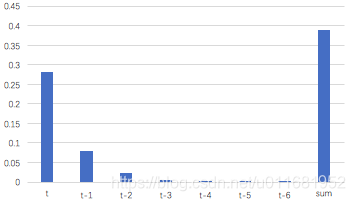
 我们就可以看到，从上图的t-3时刻开始，梯度已经几乎减少到0了。那么，从这个时刻开始再往之前走，得到的梯度（几乎为零）就不会对最终的梯度值有任何贡献，这就相当于无论t-3时刻之前的网络状态h是什么，在训练中都不会对权重数组W的更新产生影响，也就是网络事实上已经忽略了t-3时刻之前的状态。这就是原始RNN无法处理长距离依赖的原因。

 既然找到了问题的原因，那么我们就能解决它。从问题的定位到解决，科学家们大概花了7、8年时间。终于有一天，Hochreiter和Schmidhuber两位科学家发明出长短时记忆网络，一举解决这个问题。

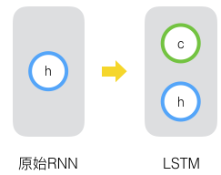
 其实，长短时记忆网络的思路比较简单。原始RNN的隐藏层只有一个状态，即h，它对于短期的输入非常敏感。那么，假如我们再增加一个状态，即c，让它来保存长期的状态，那么问题不就解决了么？如下图所示：

 新增加的状态c，称为单元状态(cell state)。我们把上图按照时间维度展开：

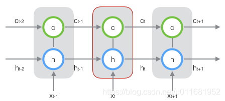
 上图仅仅是一个示意图，我们可以看出，在t时刻，LSTM的输入有三个：当前时刻网络的输入值${\mathbf{x}}_t$、上一时刻LSTM的输出值${\mathbf{h}}_{t-1}$、以及上一时刻的单元状态${\mathbf{c}}_{t-1}$；LSTM的输出有两个${\mathbf{h}}_t$：当前时刻LSTM输出值${\mathbf{c}}_t$、和当前时刻的单元状态。注意$x$、$h$、$c$都是向量。

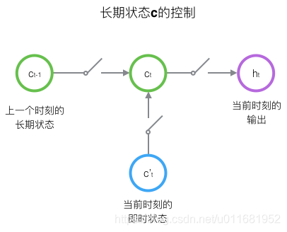
 LSTM的关键，就是怎样控制长期状态c。在这里，LSTM的思路是使用三个控制开关。第一个开关，负责控制继续保存长期状态c；第二个开关，负责控制把即时状态输入到长期状态c；第三个开关，负责控制是否把长期状态c作为当前的LSTM的输出。三个开关的作用如下图所示：

 接下来，我们要描述一下，输出h和单元状态c的具体计算方法。

3 长短时记忆网络的前向计算

 前面描述的开关是怎样在算法中实现的呢？这就用到了门（gate）的概念。门实际上就是一层全连接层，它的输入是一个向量，输出是一个0到1之间的实数向量。假设W是门的权重向量，$b$是偏置项，那么门可以表示为：
$$g(\mathbf{x})=\sigma (W\mathbf{x}+\mathbf{b})$$

 门的使用，就是用门的输出向量按元素乘以我们需要控制的那个向量。因为门的输出是0到1之间的实数向量，那么，当门输出为0时，任何向量与之相乘都会得到0向量，这就相当于啥都不能通过；输出为1时，任何向量与之相乘都不会有任何改变，这就相当于啥都可以通过。因为$\sigma$（也就是sigmoid函数）的值域是(0,1)，所以门的状态都是半开半闭的。

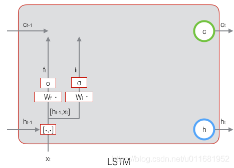
 LSTM用两个门来控制单元状态c的内容，一个是遗忘门（forget gate），它决定了上一时刻的单元状态${\mathbf{c}}_{t-1}$有多少保留到当前时刻${\mathbf{c}}_t$；另一个是输入门（input gate），它决定了当前时刻网络的输入${\mathbf{x}}_t$有多少保存到单元状态${\mathbf{c}}_t$。LSTM用输出门（output gate）来控制单元状态${\mathbf{c}}_t$有多少输出到LSTM的当前输出值${\mathbf{h}}_t$。

 我们先来看一下遗忘门：
$${\mathbf{f}}_t=\sigma (W_f\cdot [{\mathbf{h}}_{t-1},{\mathbf{x}}_t]+{\mathbf{b}}_f)(式1)$$

 上式中，$W_f$是遗忘门的权重矩阵，$[{\mathbf{h}}_{t-1},{\mathbf{x}}_t]$表示把两个向量连接成一个更长的向量，${\mathbf{b}}_f$是遗忘门的偏置项，$\sigma$是sigmoid函数。如果输入的维度是$d_x$，隐藏层的维度是$d_h$，单元状态的维度是$d_x$（通常$d_c=d_h$），则遗忘门的权重矩阵$W_f$维度是$d_c\times (d_h+d_x)$。事实上，$W_f$权重矩阵都是两个矩阵拼接而成的：一个是$W_{fh}$，它对应着输入项${\mathbf{h}}_{t-1}$，其维度为$d_c\times d_h$；一个是$W_{fx}$，它对应着输入项${\mathbf{x}}_t$，其维度为$d_c\times d_x$。$W_f$可以写为：
$$\begin{array}{rl}\left[\begin{array}{c}{W}_f\end{array}\right]\left[\begin{array}{c}{\mathbf{h}}_{t-1}\\ {\mathbf{x}}_t\end{array}\right]& =\left[\begin{array}{cc}{W}_{fh}& W_{fx}\end{array}\right]\left[\begin{array}{c}{\mathbf{h}}_{t-1}\\ {\mathbf{x}}_t\end{array}\right]\\ & =W_{fh}{\mathbf{h}}_{t-1}+W_{fx}{\mathbf{x}}_t\end{array}$$

 下图显示了遗忘门的计算：

 接下来看看输入门：
$${\mathbf{i}}_t=\sigma (W_i\cdot [{\mathbf{h}}_{t-1},{\mathbf{x}}_t]+{\mathbf{b}}_i)(式2)$$

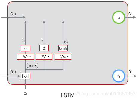
 上式中，$W_i$是输入门的权重矩阵，$b_i$是输入门的偏置项。下图表示了输入门的计算：

 接下来，我们计算用于描述当前输入的单元状态${\tilde{\mathbf{c}}}_t$，它是根据上一次的输出和本次输入来计算的：
$${\tilde{\mathbf{c}}}_t=\tanh (W_c\cdot [{\mathbf{h}}_{t-1},{\mathbf{x}}_t]+{\mathbf{b}}_c)(式3)$$
下图是${\tilde{\mathbf{c}}}_t$的计算：

 现在，我们计算当前时刻的单元状态${\mathbf{c}}_t$。它是由上一次的单元状态${\mathbf{c}}_{t-1}$按元素乘以遗忘门$f_t$，再用当前输入的单元状态${\tilde{\mathbf{c}}}_t$按元素乘以输入门$i_t$，再将两个积加和产生的：
$${\mathbf{c}}_t=f_t\circ {\mathbf{c}}_{t-1}+i_t\circ {\tilde{\mathbf{c}}}_t(式4)$$

 符号$\circ$表示按元素乘。下图是${\mathbf{c}}_t$的计算：

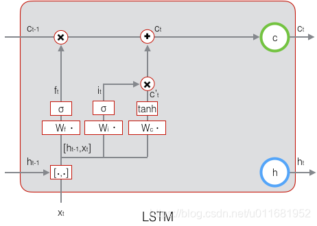
 这样，我们就把LSTM关于当前的记忆${\tilde{\mathbf{c}}}_t$和长期的记忆${\mathbf{c}}_{t-1}$组合在一起，形成了新的单元状态${\mathbf{c}}_t$。由于遗忘门的控制，它可以保存很久很久之前的信息，由于输入门的控制，它又可以避免当前无关紧要的内容进入记忆。下面，我们要看看输出门，它控制了长期记忆对当前输出的影响：
$${\mathbf{o}}_t=\sigma (W_o\cdot [{\mathbf{h}}_{t-1},{\mathbf{x}}_t]+{\mathbf{b}}_o)(式5)$$

 下图表示输出门的计算：

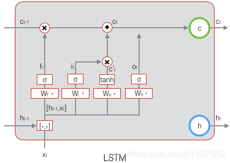
 LSTM最终的输出，是由输出门和单元状态共同确定的：
$${\mathbf{h}}_t={\mathbf{o}}_t\circ \tanh ({\mathbf{c}}_t)(式6)$$

 下图表示LSTM最终输出的计算：

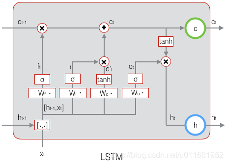
 式1到式6就是LSTM前向计算的全部公式。至此，我们就把LSTM前向计算讲完了。

4 长短时记忆网络的训练

 熟悉我们这个系列文章的同学都清楚，训练部分往往比前向计算部分复杂多了。LSTM的前向计算都这么复杂，那么，可想而知，它的训练算法一定是非常非常复杂的。现在只有做几次深呼吸，再一头扎进公式海洋吧。

4.1 LSTM训练算法框架

 LSTM的训练算法仍然是反向传播算法，对于这个算法，我们已经非常熟悉了。主要有下面三个步骤：

1. 前向计算每个神经元的输出值，对于LSTM来说，即${\mathbf{f}}_t$、${\mathbf{i}}_t$、${\mathbf{c}}_t$、${\mathbf{o}}_t$、${\mathbf{h}}_t$五个向量的值。计算方法已经在上一节中描述过了。
2. 反向计算每个神经元的误差项$\delta$值。与循环神经网络一样，LSTM误差项的反向传播也是包括两个方向：一个是沿时间的反向传播，即从当前t时刻开始，计算每个时刻的误差项；一个是将误差项向上一层传播。
3. 根据相应的误差项，计算每个权重的梯度。

4.2 关于公式和符号的说明

 首先，我们对推导中用到的一些公式、符号做一下必要的说明。

 接下来的推导中，我们设定gate的激活函数为sigmoid函数，输出的激活函数为tanh函数。他们的导数分别为：
$$\begin{array}{rl}\sigma (z)& =y=\frac{1}{1+e^{-z}}\\ {\sigma }^{\prime }(z)& =y(1-y)\\ \tanh (z)& =y=\frac{e^z-e^{-z}}{e^z+e^{-z}}\\ {\tanh }^{\prime }(z)& =1-y^2\end{array}$$

 从上面可以看出，sigmoid和tanh函数的导数都是原函数的函数。这样，我们一旦计算原函数的值，就可以用它来计算出导数的值。

 LSTM需要学习的参数共有8组，分别是：

• 遗忘门的权重矩阵$W_f$和偏置项$b_f$
• 输入门的权重矩阵$W_i$和偏置项$b_i$
• 输出门的权重矩阵$W_o$和偏置项$b_o$
• 计算单元状态的权重矩阵$W_c$和偏置项$b_c$

 因为权重矩阵的两部分在反向传播中使用不同的公式，因此在后续的推导中，权重矩阵$W_f$、$W_i$、$W_o$、$W_c$都将被写为分开的两个矩阵：$W_{fh}$、$W_{fx}$、$W_{ih}$、$W_{ix}$、$W_{oh}$、$W_{ox}$、$W_{ch}$、$W_{cx}$。

 我们解释一下按元素乘$\circ$符号。当$\circ$作用于两个向量时，运算如下：
$$\mathbf{a}\circ \mathbf{b}=\left[\begin{array}{c}{a}_1\\ a_2\\ a_3\\ ...\\ a_n\end{array}\right]\circ \left[\begin{array}{c}{b}_1\\ b_2\\ b_3\\ ...\\ b_n\end{array}\right]=\left[\begin{array}{c}{a}_1{b}_1\\ a_2{b}_2\\ a_3{b}_3\\ ...\\ a_n{b}_n\end{array}\right]$$

 当$\circ$作用于一个向量和一个矩阵时，运算如下：
$$\begin{array}{rl}\mathbf{a}\circ X& =\left[\begin{array}{c}{a}_1\\ a_2\\ a_3\\ ...\\ a_n\end{array}\right]\circ \left[\begin{array}{ccccc}{x}_{11}& x_{12}& x_{13}& ...& x_{1n}\\ x_{21}& x_{22}& x_{23}& ...& x_{2n}\\ x_{31}& x_{32}& x_{33}& ...& x_{3n}\\ & & ...& & \\ x_{n1}& x_{n2}& x_{n3}& ...& x_{nn}\end{array}\right]\\ & =\left[\begin{array}{ccccc}{a}_1{x}_{11}& a_1{x}_{12}& a_1{x}_{13}& ...& a_1{x}_{1n}\\ a_2{x}_{21}& a_2{x}_{22}& a_2{x}_{23}& ...& a_2{x}_{2n}\\ a_3{x}_{31}& a_3{x}_{32}& a_3{x}_{33}& ...& a_3{x}_{3n}\\ & & ...& & \\ a_n{x}_{n1}& a_n{x}_{n2}& a_n{x}_{n3}& ...& a_n{x}_{nn}\end{array}\right]\end{array}$$

 当$\circ$作用于两个矩阵时，两个矩阵对应位置的元素相乘。按元素乘可以在某些情况下简化矩阵和向量运算。例如，当一个对角矩阵右乘一个矩阵时，相当于用对角矩阵的对角线组成的向量按元素乘那个矩阵：
$$diag[\mathbf{a}]X=\mathbf{a}\circ X$$

 当一个行向量右乘一个对角矩阵时，相当于这个行向量按元素乘那个矩阵对角线组成的向量：
$${\mathbf{a}}^{T}diag[\mathbf{b}]=\mathbf{a}\circ \mathbf{b}$$

 上面这两点，在我们后续推导中会多次用到。

 在t时刻，LSTM的输出值为${\mathbf{h}}_t$。我们定义t时刻的误差项${\delta }_t$为：
$${\delta }_t\stackrel{def}{=}\frac{\partial E}{\partial {\mathbf{h}}_t}$$

 注意，和前面几篇文章不同，我们这里假设误差项是损失函数对输出值的导数，而不是对加权输入$ne{t}_t^l$的导数。因为LSTM有四个加权输入，分别对应${\mathbf{f}}_t$、${\mathbf{i}}_t$、${\mathbf{c}}_t$、${\mathbf{o}}_t$，我们希望往上一层传递一个误差项而不是四个。但我们仍然需要定义出这四个加权输入，以及他们对应的误差项。
$$\begin{array}{rl}{\mathbf{n}\mathbf{e}\mathbf{t}}_{f,t}& =W_f[{\mathbf{h}}_{t-1},{\mathbf{x}}_t]+{\mathbf{b}}_f\\ & =W_{fh}{\mathbf{h}}_{t-1}+W_{fx}{\mathbf{x}}_t+{\mathbf{b}}_f\\ {\mathbf{n}\mathbf{e}\mathbf{t}}_{i,t}& =W_i[{\mathbf{h}}_{t-1},{\mathbf{x}}_t]+{\mathbf{b}}_i\\ & =W_{ih}{\mathbf{h}}_{t-1}+W_{ix}{\mathbf{x}}_t+{\mathbf{b}}_i\\ {\mathbf{n}\mathbf{e}\mathbf{t}}_{\tilde{c},t}& =W_c[{\mathbf{h}}_{t-1},{\mathbf{x}}_t]+{\mathbf{b}}_c\\ & =W_{ch}{\mathbf{h}}_{t-1}+W_{cx}{\mathbf{x}}_t+{\mathbf{b}}_c\\ {\mathbf{n}\mathbf{e}\mathbf{t}}_{o,t}& =W_o[{\mathbf{h}}_{t-1},{\mathbf{x}}_t]+{\mathbf{b}}_o\\ & =W_{oh}{\mathbf{h}}_{t-1}+W_{ox}{\mathbf{x}}_t+{\mathbf{b}}_o\\ {\delta }_{f,t}& \stackrel{def}{=}\frac{\partial E}{\partial {\mathbf{n}\mathbf{e}\mathbf{t}}_{f,t}}\\ {\delta }_{i,t}& \stackrel{def}{=}\frac{\partial E}{\partial {\mathbf{n}\mathbf{e}\mathbf{t}}_{i,t}}\\ {\delta }_{\tilde{c},t}& \stackrel{def}{=}\frac{\partial E}{\partial {\mathbf{n}\mathbf{e}\mathbf{t}}_{\tilde{c},t}}\\ {\delta }_{o,t}& \stackrel{def}{=}\frac{\partial E}{\partial {\mathbf{n}\mathbf{e}\mathbf{t}}_{o,t}}\end{array}$$

4.3 误差项沿时间的反向传递

 沿时间反向传递误差项，就是要计算出t-1时刻的误差项${\delta }_{t-1}$。
$$\begin{array}{rl}{\delta }_{t-1}^T& =\frac{\partial E}{\partial {\mathbf{h}}_{\mathbf{t}-1}}\\ & =\frac{\partial E}{\partial {\mathbf{h}}_{\mathbf{t}}}\frac{\partial {\mathbf{h}}_{\mathbf{t}}}{\partial {\mathbf{h}}_{\mathbf{t}-1}}\\ & ={\delta }_t^T\frac{\partial {\mathbf{h}}_{\mathbf{t}}}{\partial {\mathbf{h}}_{\mathbf{t}-1}}\end{array}$$

 我们知道，$\frac{\partial {\mathbf{h}}_{\mathbf{t}}}{\partial {\mathbf{h}}_{\mathbf{t}-1}}$是一个Jacobian矩阵。如果隐藏层h的维度是N的话，那么它就是一个$N\times N$矩阵。为了求出它，我们列出${\mathbf{h}}_t$的计算公式，即前面的式6和式4：
$$\begin{array}{rl}{\mathbf{h}}_t& ={\mathbf{o}}_t\circ \tanh ({\mathbf{c}}_t)\\ {\mathbf{c}}_t& ={\mathbf{f}}_t\circ {\mathbf{c}}_{t-1}+{\mathbf{i}}_t\circ {\tilde{\mathbf{c}}}_t\end{array}$$

 显然，${\mathbf{o}}_t$、${\mathbf{f}}_t$、${\mathbf{i}}_t$、${\tilde{\mathbf{c}}}_t$都是${\mathbf{h}}_{t-1}$的函数，那么，利用全导数公式可得：
$$\begin{array}{rl}{\delta }_t^T\frac{\partial {\mathbf{h}}_{\mathbf{t}}}{\partial {\mathbf{h}}_{\mathbf{t}-1}}& ={\delta }_t^T\frac{\partial {\mathbf{h}}_{\mathbf{t}}}{\partial {\mathbf{o}}_t}\frac{\partial {\mathbf{o}}_t}{\partial {\mathbf{n}\mathbf{e}\mathbf{t}}_{o,t}}\frac{\partial {\mathbf{n}\mathbf{e}\mathbf{t}}_{o,t}}{\partial {\mathbf{h}}_{\mathbf{t}-1}}+{\delta }_t^T\frac{\partial {\mathbf{h}}_{\mathbf{t}}}{\partial {\mathbf{c}}_t}\frac{\partial {\mathbf{c}}_t}{\partial {\mathbf{f}}_{\mathbf{t}}}\frac{\partial {\mathbf{f}}_t}{\partial {\mathbf{n}\mathbf{e}\mathbf{t}}_{f,t}}\frac{\partial {\mathbf{n}\mathbf{e}\mathbf{t}}_{f,t}}{\partial {\mathbf{h}}_{\mathbf{t}-1}}+{\delta }_t^T\frac{\partial {\mathbf{h}}_{\mathbf{t}}}{\partial {\mathbf{c}}_t}\frac{\partial {\mathbf{c}}_t}{\partial {\mathbf{i}}_{\mathbf{t}}}\frac{\partial {\mathbf{i}}_t}{\partial {\mathbf{n}\mathbf{e}\mathbf{t}}_{i,t}}\frac{\partial {\mathbf{n}\mathbf{e}\mathbf{t}}_{i,t}}{\partial {\mathbf{h}}_{\mathbf{t}-1}}+{\delta }_t^T\frac{\partial {\mathbf{h}}_{\mathbf{t}}}{\partial {\mathbf{c}}_t}\frac{\partial {\mathbf{c}}_t}{\partial {\tilde{\mathbf{c}}}_t}\frac{\partial {\tilde{\mathbf{c}}}_t}{\partial {\mathbf{n}\mathbf{e}\mathbf{t}}_{\tilde{c},t}}\frac{\partial {\mathbf{n}\mathbf{e}\mathbf{t}}_{\tilde{c},t}}{\partial {\mathbf{h}}_{\mathbf{t}-1}}\\ & ={\delta }_{o,t}^T\frac{\partial {\mathbf{n}\mathbf{e}\mathbf{t}}_{o,t}}{\partial {\mathbf{h}}_{\mathbf{t}-1}}+{\delta }_{f,t}^T\frac{\partial {\mathbf{n}\mathbf{e}\mathbf{t}}_{f,t}}{\partial {\mathbf{h}}_{\mathbf{t}-1}}+{\delta }_{i,t}^T\frac{\partial {\mathbf{n}\mathbf{e}\mathbf{t}}_{i,t}}{\partial {\mathbf{h}}_{\mathbf{t}-1}}+{\delta }_{\tilde{c},t}^T\frac{\partial {\mathbf{n}\mathbf{e}\mathbf{t}}_{\tilde{c},t}}{\partial {\mathbf{h}}_{\mathbf{t}-1}}(式7)\end{array}$$

 下面，我们要把式7中的每个偏导数都求出来。根据式6，我们可以求出：
$$\begin{array}{rl}\frac{\partial {\mathbf{h}}_{\mathbf{t}}}{\partial {\mathbf{o}}_t}& =diag[\tanh ({\mathbf{c}}_t)]\\ \frac{\partial {\mathbf{h}}_{\mathbf{t}}}{\partial {\mathbf{c}}_t}& =diag[{\mathbf{o}}_t\circ (1-\tanh ({\mathbf{c}}_t{)}^2)]\end{array}$$

 根据式4，我们可以求出：
$$\begin{array}{rl}\frac{\partial {\mathbf{c}}_t}{\partial {\mathbf{f}}_{\mathbf{t}}}& =diag[{\mathbf{c}}_{t-1}]\\ \frac{\partial {\mathbf{c}}_t}{\partial {\mathbf{i}}_{\mathbf{t}}}& =diag[{\tilde{\mathbf{c}}}_t]\\ \frac{\partial {\mathbf{c}}_t}{\partial {\tilde{\mathbf{c}}}_{\mathbf{t}}}& =diag[{\mathbf{i}}_t]\end{array}$$

 因为：
$$\begin{array}{rl}{\mathbf{o}}_t& =\sigma ({\mathbf{n}\mathbf{e}\mathbf{t}}_{o,t})\\ {\mathbf{n}\mathbf{e}\mathbf{t}}_{o,t}& =W_{oh}{\mathbf{h}}_{t-1}+W_{ox}{\mathbf{x}}_t+{\mathbf{b}}_o\\ & \\ {\mathbf{f}}_t& =\sigma ({\mathbf{n}\mathbf{e}\mathbf{t}}_{f,t})\\ {\mathbf{n}\mathbf{e}\mathbf{t}}_{f,t}& =W_{fh}{\mathbf{h}}_{t-1}+W_{fx}{\mathbf{x}}_t+{\mathbf{b}}_f\\ & \\ {\mathbf{i}}_t& =\sigma ({\mathbf{n}\mathbf{e}\mathbf{t}}_{i,t})\\ {\mathbf{n}\mathbf{e}\mathbf{t}}_{i,t}& =W_{ih}{\mathbf{h}}_{t-1}+W_{ix}{\mathbf{x}}_t+{\mathbf{b}}_i\\ & \\ {\tilde{\mathbf{c}}}_t& =\tanh ({\mathbf{n}\mathbf{e}\mathbf{t}}_{\tilde{c},t})\\ {\mathbf{n}\mathbf{e}\mathbf{t}}_{\tilde{c},t}& =W_{ch}{\mathbf{h}}_{t-1}+W_{cx}{\mathbf{x}}_t+{\mathbf{b}}_c\end{array}$$

 我们很容易得出：
$$\begin{array}{rl}\frac{\partial {\mathbf{o}}_t}{\partial {\mathbf{n}\mathbf{e}\mathbf{t}}_{o,t}}& =diag[{\mathbf{o}}_t\circ (1-{\mathbf{o}}_t)]\\ \frac{\partial {\mathbf{n}\mathbf{e}\mathbf{t}}_{o,t}}{\partial {\mathbf{h}}_{\mathbf{t}-1}}& =W_{oh}\\ \frac{\partial {\mathbf{f}}_t}{\partial {\mathbf{n}\mathbf{e}\mathbf{t}}_{f,t}}& =diag[{\mathbf{f}}_t\circ (1-{\mathbf{f}}_t)]\\ \frac{\partial {\mathbf{n}\mathbf{e}\mathbf{t}}_{f,t}}{\partial {\mathbf{h}}_{t-1}}& =W_{fh}\\ \frac{\partial {\mathbf{i}}_t}{\partial {\mathbf{n}\mathbf{e}\mathbf{t}}_{i,t}}& =diag[{\mathbf{i}}_t\circ (1-{\mathbf{i}}_t)]\\ \frac{\partial {\mathbf{n}\mathbf{e}\mathbf{t}}_{i,t}}{\partial {\mathbf{h}}_{t-1}}& =W_{ih}\\ \frac{\partial {\tilde{\mathbf{c}}}_t}{\partial {\mathbf{n}\mathbf{e}\mathbf{t}}_{\tilde{c},t}}& =diag[1-{\tilde{\mathbf{c}}}_t^2]\\ \frac{\partial {\mathbf{n}\mathbf{e}\mathbf{t}}_{\tilde{c},t}}{\partial {\mathbf{h}}_{t-1}}& =W_{ch}\end{array}$$

 将上述偏导数带入到式7，我们得到：
$$\begin{array}{rl}{\delta }_{t-1}& ={\delta }_{o,t}^T\frac{\partial {\mathbf{n}\mathbf{e}\mathbf{t}}_{o,t}}{\partial {\mathbf{h}}_{\mathbf{t}-1}}+{\delta }_{f,t}^T\frac{\partial {\mathbf{n}\mathbf{e}\mathbf{t}}_{f,t}}{\partial {\mathbf{h}}_{\mathbf{t}-1}}+{\delta }_{i,t}^T\frac{\partial {\mathbf{n}\mathbf{e}\mathbf{t}}_{i,t}}{\partial {\mathbf{h}}_{\mathbf{t}-1}}+{\delta }_{\tilde{c},t}^T\frac{\partial {\mathbf{n}\mathbf{e}\mathbf{t}}_{\tilde{c},t}}{\partial {\mathbf{h}}_{\mathbf{t}-1}}\\ & ={\delta }_{o,t}^T{W}_{oh}+{\delta }_{f,t}^T{W}_{fh}+{\delta }_{i,t}^T{W}_{ih}+{\delta }_{\tilde{c},t}^T{W}_{ch}(式8)\end{array}$$

 根据${\delta }_{o,t}$、${\delta }_{f,t}$、${\delta }_{i,t}$、${\delta }_{\tilde{c},t}$的定义，可知：
$$\begin{array}{rl}{\delta }_{o,t}^T& ={\delta }_t^T\circ \tanh ({\mathbf{c}}_t)\circ {\mathbf{o}}_t\circ (1-{\mathbf{o}}_t)(式9)\\ {\delta }_{f,t}^T& ={\delta }_t^T\circ {\mathbf{o}}_t\circ (1-\tanh ({\mathbf{c}}_t{)}^2)\circ {\mathbf{c}}_{t-1}\circ {\mathbf{f}}_t\circ (1-{\mathbf{f}}_t)(式10)\\ {\delta }_{i,t}^T& ={\delta }_t^T\circ {\mathbf{o}}_t\circ (1-\tanh ({\mathbf{c}}_t{)}^2)\circ {\tilde{\mathbf{c}}}_t\circ {\mathbf{i}}_t\circ (1-{\mathbf{i}}_t)(式11)\\ {\delta }_{\tilde{c},t}^T& ={\delta }_t^T\circ {\mathbf{o}}_t\circ (1-\tanh ({\mathbf{c}}_t{)}^2)\circ {\mathbf{i}}_t\circ (1-{\tilde{\mathbf{c}}}^2)(式12)\end{array}$$
 式8到式12就是将误差沿时间反向传播一个时刻的公式。有了它，我们可以写出将误差项向前传递到任意k时刻的公式：
$${\delta }_k^T=\prod _{j=k}^{t-1}{\delta }_{o,j}^T{W}_{oh}+{\delta }_{f,j}^T{W}_{fh}+{\delta }_{i,j}^T{W}_{ih}+{\delta }_{\tilde{c},j}^T{W}_{ch}(式13)$$

4.4 将误差项传递到上一层

 我们假设当前为第l层，定义l-1层的误差项是误差函数对l-1层加权输入的导数，即：
$${\delta }_t^{l-1}\stackrel{def}{=}\frac{\partial E}{{\mathbf{n}\mathbf{e}\mathbf{t}}_t^{l-1}}$$

 本次LSTM的输入$x_t$由下面的公式计算：
$${\mathbf{x}}_t^l=f^{l-1}({\mathbf{n}\mathbf{e}\mathbf{t}}_t^{l-1})$$

 上式中，$f^{l-1}$表示第l-1层的激活函数。

 因为${\mathbf{n}\mathbf{e}\mathbf{t}}_{f,t}^l$、${\mathbf{n}\mathbf{e}\mathbf{t}}_{i,t}^l$、${\mathbf{n}\mathbf{e}\mathbf{t}}_{\tilde{c},t}^l$、${\mathbf{n}\mathbf{e}\mathbf{t}}_{o,t}^l$都是${\mathbf{x}}_t$的函数，${\mathbf{x}}_t$又是${\mathbf{n}\mathbf{e}\mathbf{t}}_t^{l-1}$的函数，因此，要求出E对${\mathbf{n}\mathbf{e}\mathbf{t}}_t^{l-1}$的导数，就需要使用全导数公式：
$$\begin{array}{rl}\frac{\partial E}{\partial {\mathbf{n}\mathbf{e}\mathbf{t}}_t^{l-1}}& =\frac{\partial E}{\partial {\mathbf{n}\mathbf{e}\mathbf{t}}_{\mathbf{f},\mathbf{t}}^{\mathbf{l}}}\frac{\partial {\mathbf{n}\mathbf{e}\mathbf{t}}_{\mathbf{f},\mathbf{t}}^{\mathbf{l}}}{\partial {\mathbf{x}}_t^l}\frac{\partial {\mathbf{x}}_t^l}{\partial {\mathbf{n}\mathbf{e}\mathbf{t}}_{\mathbf{t}}^{\mathbf{l}-1}}+\frac{\partial E}{\partial {\mathbf{n}\mathbf{e}\mathbf{t}}_{\mathbf{i},\mathbf{t}}^{\mathbf{l}}}\frac{\partial {\mathbf{n}\mathbf{e}\mathbf{t}}_{\mathbf{i},\mathbf{t}}^{\mathbf{l}}}{\partial {\mathbf{x}}_t^l}\frac{\partial {\mathbf{x}}_t^l}{\partial {\mathbf{n}\mathbf{e}\mathbf{t}}_{\mathbf{t}}^{\mathbf{l}-1}}+\frac{\partial E}{\partial {\mathbf{n}\mathbf{e}\mathbf{t}}_{\tilde{\mathbf{c}},\mathbf{t}}^{\mathbf{l}}}\frac{\partial {\mathbf{n}\mathbf{e}\mathbf{t}}_{\tilde{\mathbf{c}},\mathbf{t}}^{\mathbf{l}}}{\partial {\mathbf{x}}_t^l}\frac{\partial {\mathbf{x}}_t^l}{\partial {\mathbf{n}\mathbf{e}\mathbf{t}}_{\mathbf{t}}^{\mathbf{l}-1}}+\frac{\partial E}{\partial {\mathbf{n}\mathbf{e}\mathbf{t}}_{\mathbf{o},\mathbf{t}}^{\mathbf{l}}}\frac{\partial {\mathbf{n}\mathbf{e}\mathbf{t}}_{\mathbf{o},\mathbf{t}}^{\mathbf{l}}}{\partial {\mathbf{x}}_t^l}\frac{\partial {\mathbf{x}}_t^l}{\partial {\mathbf{n}\mathbf{e}\mathbf{t}}_{\mathbf{t}}^{\mathbf{l}-1}}\\ & ={\delta }_{f,t}^T{W}_{fx}\circ f^{\prime }({\mathbf{n}\mathbf{e}\mathbf{t}}_t^{l-1})+{\delta }_{i,t}^T{W}_{ix}\circ f^{\prime }({\mathbf{n}\mathbf{e}\mathbf{t}}_t^{l-1})+{\delta }_{\tilde{c},t}^T{W}_{cx}\circ f^{\prime }({\mathbf{n}\mathbf{e}\mathbf{t}}_t^{l-1})+{\delta }_{o,t}^T{W}_{ox}\circ f^{\prime }({\mathbf{n}\mathbf{e}\mathbf{t}}_t^{l-1})\\ & =({\delta }_{f,t}^T{W}_{fx}+{\delta }_{i,t}^T{W}_{ix}+{\delta }_{\tilde{c},t}^T{W}_{cx}+{\delta }_{o,t}^T{W}_{ox})\circ f^{\prime }({\mathbf{n}\mathbf{e}\mathbf{t}}_t^{l-1})(式14)\end{array}$$

 式14就是将误差传递到上一层的公式。

4.5 权重梯度的计算

 对于$W_{fh}$、$W_{ih}$、$W_{ch}$、$W_{oh}$的权重梯度，我们知道它的梯度是各个时刻梯度之和（证明过程请参考文章零基础入门深度学习(5) - 循环神经网络），我们首先求出它们在t时刻的梯度，然后再求出他们最终的梯度。

 我们已经求得了误差项${\delta }_{o,t}$、${\delta }_{f,t}$、${\delta }_{i,t}$、${\delta }_{\tilde{c},t}$，很容易求出t时刻的$W_{fh}$、$W_{ih}$、$W_{ch}$、$W_{oh}$：
$$\begin{array}{rl}\frac{\partial E}{\partial W_{oh,t}}& =\frac{\partial E}{\partial {\mathbf{n}\mathbf{e}\mathbf{t}}_{o,t}}\frac{\partial {\mathbf{n}\mathbf{e}\mathbf{t}}_{o,t}}{\partial W_{oh,t}}\\ & ={\delta }_{o,t}{\mathbf{h}}_{t-1}^T\\ & \\ \frac{\partial E}{\partial W_{fh,t}}& =\frac{\partial E}{\partial {\mathbf{n}\mathbf{e}\mathbf{t}}_{f,t}}\frac{\partial {\mathbf{n}\mathbf{e}\mathbf{t}}_{f,t}}{\partial W_{fh,t}}\\ & ={\delta }_{f,t}{\mathbf{h}}_{t-1}^T\\ & \\ \frac{\partial E}{\partial W_{ih,t}}& =\frac{\partial E}{\partial {\mathbf{n}\mathbf{e}\mathbf{t}}_{i,t}}\frac{\partial {\mathbf{n}\mathbf{e}\mathbf{t}}_{i,t}}{\partial W_{ih,t}}\\ & ={\delta }_{i,t}{\mathbf{h}}_{t-1}^T\\ & \\ \frac{\partial E}{\partial W_{ch,t}}& =\frac{\partial E}{\partial {\mathbf{n}\mathbf{e}\mathbf{t}}_{\tilde{c},t}}\frac{\partial {\mathbf{n}\mathbf{e}\mathbf{t}}_{\tilde{c},t}}{\partial W_{ch,t}}\\ & ={\delta }_{\tilde{c},t}{\mathbf{h}}_{t-1}^T\end{array}$$

 将各个时刻的梯度加在一起，就能得到最终的梯度：
$$\begin{array}{rl}\frac{\partial E}{\partial W_{oh}}& =\sum _{j=1}^t{\delta }_{o,j}{\mathbf{h}}_{j-1}^T\\ \frac{\partial E}{\partial W_{fh}}& =\sum _{j=1}^t{\delta }_{f,j}{\mathbf{h}}_{j-1}^T\\ \frac{\partial E}{\partial W_{ih}}& =\sum _{j=1}^t{\delta }_{i,j}{\mathbf{h}}_{j-1}^T\\ \frac{\partial E}{\partial W_{ch}}& =\sum _{j=1}^t{\delta }_{\tilde{c},j}{\mathbf{h}}_{j-1}^T\end{array}$$

 对于偏置项${\mathbf{b}}_f$、${\mathbf{b}}_i$、${\mathbf{b}}_c$、${\mathbf{b}}_o$的梯度，也是将各个时刻的梯度加在一起。下面是各个时刻的偏置项梯度：
$$\begin{array}{rl}\frac{\partial E}{\partial {\mathbf{b}}_{o,t}}& =\frac{\partial E}{\partial {\mathbf{n}\mathbf{e}\mathbf{t}}_{o,t}}\frac{\partial {\mathbf{n}\mathbf{e}\mathbf{t}}_{o,t}}{\partial {\mathbf{b}}_{o,t}}\\ & ={\delta }_{o,t}\\ & \\ \frac{\partial E}{\partial {\mathbf{b}}_{f,t}}& =\frac{\partial E}{\partial {\mathbf{n}\mathbf{e}\mathbf{t}}_{f,t}}\frac{\partial {\mathbf{n}\mathbf{e}\mathbf{t}}_{f,t}}{\partial {\mathbf{b}}_{f,t}}\\ & ={\delta }_{f,t}\\ & \\ \frac{\partial E}{\partial {\mathbf{b}}_{i,t}}& =\frac{\partial E}{\partial {\mathbf{n}\mathbf{e}\mathbf{t}}_{i,t}}\frac{\partial {\mathbf{n}\mathbf{e}\mathbf{t}}_{i,t}}{\partial {\mathbf{b}}_{i,t}}\\ & ={\delta }_{i,t}\\ & \\ \frac{\partial E}{\partial {\mathbf{b}}_{c,t}}& =\frac{\partial E}{\partial {\mathbf{n}\mathbf{e}\mathbf{t}}_{\tilde{c},t}}\frac{\partial {\mathbf{n}\mathbf{e}\mathbf{t}}_{\tilde{c},t}}{\partial {\mathbf{b}}_{c,t}}\\ & ={\delta }_{\tilde{c},t}\end{array}$$

 下面是最终的偏置项梯度，即将各个时刻的偏置项梯度加在一起：
$$\begin{array}{rl}\frac{\partial E}{\partial {\mathbf{b}}_o}& =\sum _{j=1}^t{\delta }_{o,j}\\ \frac{\partial E}{\partial {\mathbf{b}}_i}& =\sum _{j=1}^t{\delta }_{i,j}\\ \frac{\partial E}{\partial {\mathbf{b}}_f}& =\sum _{j=1}^t{\delta }_{f,j}\\ \frac{\partial E}{\partial {\mathbf{b}}_c}& =\sum _{j=1}^t{\delta }_{\tilde{c},j}\end{array}$$

 对于$W_{fx}$、$W_{ix}$、$W_{cx}$、$W_{ox}$的权重梯度，只需要根据相应的误差项直接计算即可：
$$\begin{array}{rl}\frac{\partial E}{\partial W_{ox}}& =\frac{\partial E}{\partial {\mathbf{n}\mathbf{e}\mathbf{t}}_{o,t}}\frac{\partial {\mathbf{n}\mathbf{e}\mathbf{t}}_{o,t}}{\partial W_{ox}}\\ & ={\delta }_{o,t}{\mathbf{x}}_t^T\\ & \\ \frac{\partial E}{\partial W_{fx}}& =\frac{\partial E}{\partial {\mathbf{n}\mathbf{e}\mathbf{t}}_{f,t}}\frac{\partial {\mathbf{n}\mathbf{e}\mathbf{t}}_{f,t}}{\partial W_{fx}}\\ & ={\delta }_{f,t}{\mathbf{x}}_t^T\\ & \\ \frac{\partial E}{\partial W_{ix}}& =\frac{\partial E}{\partial {\mathbf{n}\mathbf{e}\mathbf{t}}_{i,t}}\frac{\partial {\mathbf{n}\mathbf{e}\mathbf{t}}_{i,t}}{\partial W_{ix}}\\ & ={\delta }_{i,t}{\mathbf{x}}_t^T\\ & \\ \frac{\partial E}{\partial W_{cx}}& =\frac{\partial E}{\partial {\mathbf{n}\mathbf{e}\mathbf{t}}_{\tilde{c},t}}\frac{\partial {\mathbf{n}\mathbf{e}\mathbf{t}}_{\tilde{c},t}}{\partial W_{cx}}\\ & ={\delta }_{\tilde{c},t}{\mathbf{x}}_t^T\end{array}$$

 以上就是LSTM的训练算法的全部公式。因为这里面存在很多重复的模式，仔细看看，会发觉并不是太复杂。

 当然，LSTM存在着相当多的变体，读者可以在互联网上找到很多资料。因为大家已经熟悉了基本LSTM的算法，因此理解这些变体比较容易，因此本文就不再赘述了。

5 长短时记忆网络的实现

 完整代码请参考GitHub: https://github.com/hanbt/learn_dl/blob/master/lstm.py (python2.7)

 在下面的实现中，LSTMLayer的参数包括输入维度、输出维度、隐藏层维度，单元状态维度等于隐藏层维度。gate的激活函数为sigmoid函数，输出的激活函数为tanh。

5.1 激活函数的实现

 我们先实现两个激活函数：sigmoid和tanh。

class SigmoidActivator(object):
    def forward(self, weighted_input):
        return 1.0 / (1.0 + np.exp(-weighted_input))
    def backward(self, output):
        return output * (1 - output)
class TanhActivator(object):
    def forward(self, weighted_input):
        return 2.0 / (1.0 + np.exp(-2 * weighted_input)) - 1.0
    def backward(self, output):
        return 1 - output * output

5.2 LSTM初始化

 和前两篇文章代码架构一样，我们把LSTM的实现放在LstmLayer类中。

 根据LSTM前向计算和方向传播算法，我们需要初始化一系列矩阵和向量。这些矩阵和向量有两类用途，一类是用于保存模型参数，例如${\mathbf{W}}_f$、${\mathbf{W}}_i$、${\mathbf{W}}_c$、${\mathbf{W}}_o$、${\mathbf{b}}_f$、${\mathbf{b}}_i$、${\mathbf{b}}_c$、${\mathbf{b}}_o$；另一类是保存各种中间计算结果，以便于反向传播算法使用，它们包括${\mathbf{h}}_t$、${\mathbf{f}}_t$、${\mathbf{i}}_t$、${\mathbf{o}}_t$、${\mathbf{c}}_t$、${\tilde{\mathbf{c}}}_t$、${\delta }_t$、${\delta }_{f,t}$、${\delta }_{i,t}$、${\delta }_{o,t}$、${\delta }_{\tilde{c},t}$，以及各个权重对应的梯度。

 在构造函数的初始化中，只初始化了与forward计算相关的变量，与backward相关的变量没有初始化。这是因为构造LSTM对象的时候，我们还不知道它未来是用于训练（既有forward又有backward）还是推理（只有forward）。

class LstmLayer(object):
    def __init__(self, input_width, state_width, 
                 learning_rate):
        self.input_width = input_width
        self.state_width = state_width
        self.learning_rate = learning_rate
        # 门的激活函数
        self.gate_activator = SigmoidActivator()
        # 输出的激活函数
        self.output_activator = TanhActivator()
        # 当前时刻初始化为t0
        self.times = 0       
        # 各个时刻的单元状态向量c
        self.c_list = self.init_state_vec()
        # 各个时刻的输出向量h
        self.h_list = self.init_state_vec()
        # 各个时刻的遗忘门f
        self.f_list = self.init_state_vec()
        # 各个时刻的输入门i
        self.i_list = self.init_state_vec()
        # 各个时刻的输出门o
        self.o_list = self.init_state_vec()
        # 各个时刻的即时状态c~
        self.ct_list = self.init_state_vec()
        # 遗忘门权重矩阵Wfh, Wfx, 偏置项bf
        self.Wfh, self.Wfx, self.bf = (
            self.init_weight_mat())
        # 输入门权重矩阵Wfh, Wfx, 偏置项bf
        self.Wih, self.Wix, self.bi = (
            self.init_weight_mat())
        # 输出门权重矩阵Wfh, Wfx, 偏置项bf
        self.Woh, self.Wox, self.bo = (
            self.init_weight_mat())
        # 单元状态权重矩阵Wfh, Wfx, 偏置项bf
        self.Wch, self.Wcx, self.bc = (
            self.init_weight_mat())
    def init_state_vec(self):
        '''
        初始化保存状态的向量
        '''
        state_vec_list = []
        state_vec_list.append(np.zeros(
            (self.state_width, 1)))
        return state_vec_list
    def init_weight_mat(self):
        '''
        初始化权重矩阵
        '''
        Wh = np.random.uniform(-1e-4, 1e-4,
            (self.state_width, self.state_width))
        Wx = np.random.uniform(-1e-4, 1e-4,
            (self.state_width, self.input_width))
        b = np.zeros((self.state_width, 1))
        return Wh, Wx, b

5.3 前向计算的实现

 forward方法实现了LSTM的前向计算：

def forward(self, x):
    '''
    根据式1-式6进行前向计算
    '''
    self.times += 1
    # 遗忘门
    fg = self.calc_gate(x, self.Wfx, self.Wfh, 
        self.bf, self.gate_activator)
    self.f_list.append(fg)
    # 输入门
    ig = self.calc_gate(x, self.Wix, self.Wih,
        self.bi, self.gate_activator)
    self.i_list.append(ig)
    # 输出门
    og = self.calc_gate(x, self.Wox, self.Woh,
        self.bo, self.gate_activator)
    self.o_list.append(og)
    # 即时状态
    ct = self.calc_gate(x, self.Wcx, self.Wch,
        self.bc, self.output_activator)
    self.ct_list.append(ct)
    # 单元状态
    c = fg * self.c_list[self.times - 1] + ig * ct
    self.c_list.append(c)
    # 输出
    h = og * self.output_activator.forward(c)
    self.h_list.append(h)
def calc_gate(self, x, Wx, Wh, b, activator):
    '''
    计算门
    '''
    h = self.h_list[self.times - 1] # 上次的LSTM输出
    net = np.dot(Wh, h) + np.dot(Wx, x) + b
    gate = activator.forward(net)
    return gate

 从上面的代码我们可以看到，门的计算都是相同的算法，而门和${\tilde{\mathbf{c}}}_{\mathbf{t}}$的计算仅仅是激活函数不同。因此我们提出了calc_gate方法，这样减少了很多重复代码。

5.4 反向传播算法的实现

 backward方法实现了LSTM的反向传播算法。需要注意的是，与backword相关的内部状态变量是在调用backward方法之后才初始化的。这种延迟初始化的一个好处是，如果LSTM只是用来推理，那么就不需要初始化这些变量，节省了很多内存。

def backward(self, x, delta_h, activator):
    '''
    实现LSTM训练算法
    '''
    self.calc_delta(delta_h, activator)
    self.calc_gradient(x)

 算法主要分成两个部分，一部分使计算误差项：

def calc_delta(self, delta_h, activator):
    # 初始化各个时刻的误差项
    self.delta_h_list = self.init_delta()  # 输出误差项
    self.delta_o_list = self.init_delta()  # 输出门误差项
    self.delta_i_list = self.init_delta()  # 输入门误差项
    self.delta_f_list = self.init_delta()  # 遗忘门误差项
    self.delta_ct_list = self.init_delta() # 即时输出误差项
    # 保存从上一层传递下来的当前时刻的误差项
    self.delta_h_list[-1] = delta_h
    # 迭代计算每个时刻的误差项
    for k in range(self.times, 0, -1):
        self.calc_delta_k(k)
def init_delta(self):
    '''
    初始化误差项
    '''
    delta_list = []
    for i in range(self.times + 1):
        delta_list.append(np.zeros(
            (self.state_width, 1)))
    return delta_list
def calc_delta_k(self, k):
    '''
    根据k时刻的delta_h，计算k时刻的delta_f、
    delta_i、delta_o、delta_ct，以及k-1时刻的delta_h
    '''
    # 获得k时刻前向计算的值
    ig = self.i_list[k]
    og = self.o_list[k]
    fg = self.f_list[k]
    ct = self.ct_list[k]
    c = self.c_list[k]
    c_prev = self.c_list[k-1]
    tanh_c = self.output_activator.forward(c)
    delta_k = self.delta_h_list[k]
    # 根据式9计算delta_o
    delta_o = (delta_k * tanh_c * 
        self.gate_activator.backward(og))
    delta_f = (delta_k * og * 
        (1 - tanh_c * tanh_c) * c_prev *
        self.gate_activator.backward(fg))
    delta_i = (delta_k * og * 
        (1 - tanh_c * tanh_c) * ct *
        self.gate_activator.backward(ig))
    delta_ct = (delta_k * og * 
        (1 - tanh_c * tanh_c) * ig *
        self.output_activator.backward(ct))
    delta_h_prev = (
            np.dot(delta_o.transpose(), self.Woh) +
            np.dot(delta_i.transpose(), self.Wih) +
            np.dot(delta_f.transpose(), self.Wfh) +
            np.dot(delta_ct.transpose(), self.Wch)
        ).transpose()
    # 保存全部delta值
    self.delta_h_list[k-1] = delta_h_prev
    self.delta_f_list[k] = delta_f
    self.delta_i_list[k] = delta_i
    self.delta_o_list[k] = delta_o
    self.delta_ct_list[k] = delta_ct

 另一部分是计算梯度：

def calc_gradient(self, x):
    # 初始化遗忘门权重梯度矩阵和偏置项
    self.Wfh_grad, self.Wfx_grad, self.bf_grad = (
        self.init_weight_gradient_mat())
    # 初始化输入门权重梯度矩阵和偏置项
    self.Wih_grad, self.Wix_grad, self.bi_grad = (
        self.init_weight_gradient_mat())
    # 初始化输出门权重梯度矩阵和偏置项
    self.Woh_grad, self.Wox_grad, self.bo_grad = (
        self.init_weight_gradient_mat())
    # 初始化单元状态权重梯度矩阵和偏置项
    self.Wch_grad, self.Wcx_grad, self.bc_grad = (
        self.init_weight_gradient_mat())
   # 计算对上一次输出h的权重梯度
    for t in range(self.times, 0, -1):
        # 计算各个时刻的梯度
        (Wfh_grad, bf_grad,
        Wih_grad, bi_grad,
        Woh_grad, bo_grad,
        Wch_grad, bc_grad) = (
            self.calc_gradient_t(t))
        # 实际梯度是各时刻梯度之和
        self.Wfh_grad += Wfh_grad
        self.bf_grad += bf_grad
        self.Wih_grad += Wih_grad
        self.bi_grad += bi_grad
        self.Woh_grad += Woh_grad
        self.bo_grad += bo_grad
        self.Wch_grad += Wch_grad
        self.bc_grad += bc_grad
        print '-----%d-----' % t
        print Wfh_grad
        print self.Wfh_grad
    # 计算对本次输入x的权重梯度
    xt = x.transpose()
    self.Wfx_grad = np.dot(self.delta_f_list[-1], xt)
    self.Wix_grad = np.dot(self.delta_i_list[-1], xt)
    self.Wox_grad = np.dot(self.delta_o_list[-1], xt)
    self.Wcx_grad = np.dot(self.delta_ct_list[-1], xt)
def init_weight_gradient_mat(self):
    '''
    初始化权重矩阵
    '''
    Wh_grad = np.zeros((self.state_width,
        self.state_width))
    Wx_grad = np.zeros((self.state_width,
        self.input_width))
    b_grad = np.zeros((self.state_width, 1))
    return Wh_grad, Wx_grad, b_grad
def calc_gradient_t(self, t):
    '''
    计算每个时刻t权重的梯度
    '''
    h_prev = self.h_list[t-1].transpose()
    Wfh_grad = np.dot(self.delta_f_list[t], h_prev)
    bf_grad = self.delta_f_list[t]
    Wih_grad = np.dot(self.delta_i_list[t], h_prev)
    bi_grad = self.delta_f_list[t]
    Woh_grad = np.dot(self.delta_o_list[t], h_prev)
    bo_grad = self.delta_f_list[t]
    Wch_grad = np.dot(self.delta_ct_list[t], h_prev)
    bc_grad = self.delta_ct_list[t]
    return Wfh_grad, bf_grad, Wih_grad, bi_grad, \
           Woh_grad, bo_grad, Wch_grad, bc_grad

5.5 梯度下降算法的实现

 下面是用梯度下降算法来更新权重：

def update(self):
    '''
    按照梯度下降，更新权重
    '''
    self.Wfh -= self.learning_rate * self.Whf_grad
    self.Wfx -= self.learning_rate * self.Whx_grad
    self.bf -= self.learning_rate * self.bf_grad
    self.Wih -= self.learning_rate * self.Whi_grad
    self.Wix -= self.learning_rate * self.Whi_grad
    self.bi -= self.learning_rate * self.bi_grad
    self.Woh -= self.learning_rate * self.Wof_grad
    self.Wox -= self.learning_rate * self.Wox_grad
    self.bo -= self.learning_rate * self.bo_grad
    self.Wch -= self.learning_rate * self.Wcf_grad
    self.Wcx -= self.learning_rate * self.Wcx_grad
    self.bc -= self.learning_rate * self.bc_grad

5.6 梯度检查的实现

 和RecurrentLayer一样，为了支持梯度检查，我们需要支持重置内部状态：

def reset_state(self):
    # 当前时刻初始化为t0
    self.times = 0       
    # 各个时刻的单元状态向量c
    self.c_list = self.init_state_vec()
    # 各个时刻的输出向量h
    self.h_list = self.init_state_vec()
    # 各个时刻的遗忘门f
    self.f_list = self.init_state_vec()
    # 各个时刻的输入门i
    self.i_list = self.init_state_vec()
    # 各个时刻的输出门o
    self.o_list = self.init_state_vec()
    # 各个时刻的即时状态c~
    self.ct_list = self.init_state_vec()

 最后，是梯度检查的代码：

def data_set():
    x = [np.array([[1], [2], [3]]),
         np.array([[2], [3], [4]])]
    d = np.array([[1], [2]])
    return x, d
def gradient_check():
    '''
    梯度检查
    '''
    # 设计一个误差函数，取所有节点输出项之和
    error_function = lambda o: o.sum()
    lstm = LstmLayer(3, 2, 1e-3)
    # 计算forward值
    x, d = data_set()
    lstm.forward(x[0])
    lstm.forward(x[1])
    # 求取sensitivity map
    sensitivity_array = np.ones(lstm.h_list[-1].shape,
                                dtype=np.float64)
    # 计算梯度
    lstm.backward(x[1], sensitivity_array, IdentityActivator())
    # 检查梯度
    epsilon = 10e-4
    for i in range(lstm.Wfh.shape[0]):
        for j in range(lstm.Wfh.shape[1]):
            lstm.Wfh[i,j] += epsilon
            lstm.reset_state()
            lstm.forward(x[0])
            lstm.forward(x[1])
            err1 = error_function(lstm.h_list[-1])
            lstm.Wfh[i,j] -= 2*epsilon
            lstm.reset_state()
            lstm.forward(x[0])
            lstm.forward(x[1])
            err2 = error_function(lstm.h_list[-1])
            expect_grad = (err1 - err2) / (2 * epsilon)
            lstm.Wfh[i,j] += epsilon
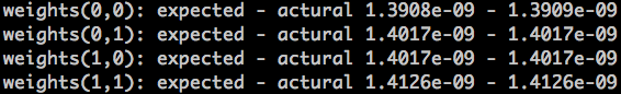
            print 'weights(%d,%d): expected - actural %.4e - %.4e' % (
                i, j, expect_grad, lstm.Wfh_grad[i,j])
    return lstm

 我们只对做了检查，读者可以自行增加对其他梯度的检查。下面是某次梯度检查的结果：

6 GRU

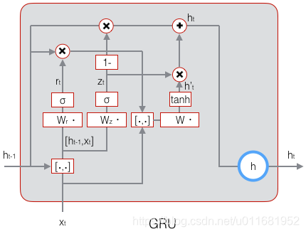
 前面我们讲了一种普通的LSTM，事实上LSTM存在很多变体，许多论文中的LSTM都或多或少的不太一样。在众多的LSTM变体中，GRU (Gated Recurrent Unit)也许是最成功的一种。它对LSTM做了很多简化，同时却保持着和LSTM相同的效果。因此，GRU最近变得越来越流行。

 GRU对LSTM做了两个大改动：

1. 将输入门、遗忘门、输出门变为两个门：更新门（Update Gate）${\mathbf{z}}_t$和重置门（Reset
   Gate）${\mathbf{r}}_t$。
2. 将单元状态与输出合并为一个状态：$h$。

 GRU的前向计算公式为：
$$\begin{array}{rl}{\mathbf{z}}_t& =\sigma (W_z\cdot [{\mathbf{h}}_{t-1},{\mathbf{x}}_t])\\ {\mathbf{r}}_t& =\sigma (W_r\cdot [{\mathbf{h}}_{t-1},{\mathbf{x}}_t])\\ {\tilde{\mathbf{h}}}_t& =\tanh (W\cdot [{\mathbf{r}}_t\circ {\mathbf{h}}_{t-1},{\mathbf{x}}_t])\\ \mathbf{h}& =(1-{\mathbf{z}}_t)\circ {\mathbf{h}}_{t-1}+{\mathbf{z}}_t\circ {\tilde{\mathbf{h}}}_t\end{array}$$

 下图是GRU的示意图：

 GRU的训练算法比LSTM简单一些，留给读者自行推导，本文就不再赘述了。

7 小结

 至此，LSTM——也许是结构最复杂的一类神经网络——就讲完了，相信拿下前几篇文章的读者们搞定这篇文章也不在话下吧！现在我们已经了解循环神经网络和它最流行的变体——LSTM，它们都可以用来处理序列。但是，有时候仅仅拥有处理序列的能力还不够，还需要处理比序列更为复杂的结构（比如树结构），这时候就需要用到另外一类网络：递归神经网络(Recursive Neural Network)，巧合的是，它的缩写也是RNN。在下一篇文章中，我们将介绍递归神经网络和它的训练算法。现在，漫长的烧脑暂告一段落，休息一下吧:)

8 参考资料

CS224d: Deep Learning for Natural Language Processing
Understanding LSTM Networks
LSTM Forward and Backward Pass