


Time series prediction problems are a difficult type of predictive modeling problem.Unlike regression predictive modeling, time series also adds the complexity of a sequence dependence among the input variables. A powerful type of neural network designed to handle sequence dependence are called recurrent neural networks. The Long Short-Term Memory Networks or LSTM network is a type of recurrent neural network used in deep learning because very large architectures can be successfully trained.
In this lesson you will discover how to develop LSTM networks in Python using the Keras deep learning library to address a demonstration time series prediction problem. After completing this tutorial you will know how to implement and develop LSTM networks for your own time series prediction problems and other more general sequence problems. You will know:
- How to develop LSTM networks for a time series prediction problem framed as regression.
- How to develop LSTM networks for a time series prediction problem using a window for both features and time steps.
- How to develop and make predictions using LSTM networks that maintain state (memory) across very long sequences.
We will develop a number of LSTMs for a standard time series prediction problem. The problem and the chosen configuration for the LSTM networks are for demonstration purposes only, they are not optimized. These examples will show you exactly how you can develop your own LSTM networks for time series predictive modeling problems. Let’s get started.
1.1 LSTM Network For Regression
The problem we are going to look at in this lesson is the international airline passengers prediction problem, described in Section 24.1. We can phrase the problem as a regression problem, as was done in the previous chapter. That is, given the number of passengers (in units of thousands) this month, what is the number of passengers next month. This example will reuse the same data loading and preparation from the previous chapter, specifically the use of the create_dataset() function.
LSTMs are sensitive to the scale of the input data, specifically when the sigmoid (default) or tanh activation functions are used. It can be a good practice to rescale the data to the range of 0-to-1, also called normalizing. We can easily normalize the dataset using the MinMaxScaler preprocessing class from the scikit-learn library.
# normalize the dataset
from sklearn.preprocessing import MinMaxScaler
scaler = MinMaxScaler(feature_range=(0, 1))
dataset = scaler.fit_transform(dataset)
The LSTM network expects the input data (X) to be provided with a specific array structure in the form of: [samples, time steps, features]. Our prepared data is in the form: [samples, features] and we are framing the problem as one time step for each sample. We can transform the prepared train and test input data into the expected structure using numpy.reshape() as follows:
# Reshape the Prepared Dataset for the LSTM Layers
# reshape input to be [samples, time step, features]
trainX = np.reshape(trainX,(trainX.shape[0], 1,trainX.shape[1]))
testX = np.reshape(testX, (testX.shape[0], 1, testX.shape[1]))
We are now ready to design and fit our LSTM network for this problem. The network has a visible layer with 1 input, a hidden layer with 4 LSTM blocks or neurons and an output layer that makes a single value prediction. The default sigmoid activation function is used for the LSTM memory blocks. The network is trained for 100 epochs and a batch size of 1 is used.
# Define and Fit the LSTM network
# create and fit the LSTM network
model = Sequential()
model.add(LSTM(4, input_dim=look_back))
model.add(Dense(1))
model.compile(loss='mean_squared_error',optimizer='adam')
model.fit(trainX,trainY, epochs=100, batch_size=1,verbose=2)
For completeness, below is the entire code example.
# LSTM for international airline passengers problem with regression framing
import numpy as np
import matplotlib.pyplot as plt
import pandas as pd
import math
from keras.models import Sequential
from keras.layers import Dense
from keras.layers import LSTM
from sklearn.preprocessing import MinMaxScaler
from sklearn.metrics import mean_squared_error
# convert an array of values into a dataset matrix
def create_dataset(dataset, look_back=1):
dataX, dataY = [],[]
for i in range(len(dataset)-look_back-1):
a = dataset[i:(i+look_back),0]
dataX.append(a)
dataY.append(dataset[i + look_back,0])
return np.array(dataX), np.array(dataY)
# fix random seed for reproducibility
seed = 7
np.random.seed(seed)
# load the dataset
dataframe = pd.read_csv('international-airline-passengers.csv',usecols=[1],engine='python',skipfooter=3)
dataset = dataframe.values
dataset = dataset.astype('float32')
# normalize the dataset
scaler = MinMaxScaler(feature_range=(0, 1))
dataset = scaler.fit_transform(dataset)
# split into train and test sets
train_size = int(len(dataset) * 0.67)
test_size = len(dataset) - train_size
train, test = dataset[0:train_size,:],dataset[train_size:len(dataset),:]
# reshape into X=t and Y=t+1
look_back = 1
trainX, trainY = create_dataset(train, look_back)
testX, testY = create_dataset(test, look_back)
# reshape input to be [samples, time steps, features]
trainX = np.reshape(trainX,(trainX.shape[0], 1, trainX.shape[1]))
testX = np.reshape(testX, (testX.shape[0], 1, testX.shape[1]))
# create and fit the LSTM network
model = Sequential()
model.add(LSTM(4, input_dim=look_back))
model.add(Dense(1))
model.compile(loss='mean_squared_error',optimizer='adam')
model.fit(trainX,trainY,epochs=100, batch_size=1,verbose=2)
# make predictions
trainPredict = model.predict(trainX)
testPredict = model.predict(testX)
#invert predictions
trainPredict = scaler.inverse_transform(trainPredict)
trainY = scaler.inverse_transform([trainY])
testPredict = scaler.inverse_transform(testPredict)
testY = scaler.inverse_transform([testY])
# calculate root mean suqared error
trainScore = math.sqrt(mean_squared_error(trainY[0],trainPredict[:,0]))
print('Train Score: %.2f%%'% (trainScore))
testScore = math.sqrt(mean_squared_error(testY[0],testPredict[:,0]))
print('Test Score: %.2f RMSE' %(testScore))
#shift train prediction for plotting
trainPredictPlot = np.empty_like(dataset)
trainPredictPlot[:, :] = np.nan
trainPredictPlot[look_back:len(trainPredict)+look_back,:] = trainPredict
# shift test predictions for plotting
testPredictPlot = np.empty_like(dataset)
testPredictPlot[:, :] = np.nan
testPredictPlot[len(trainPredict)+(look_back*2)+1:len(dataset)-1, :] = testPredict
# plot baseline and predictions
plt.plot(scaler.inverse_transform(dataset))
plt.plot(trainPredictPlot)
plt.plot(testPredictPlot)
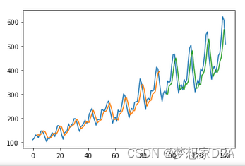
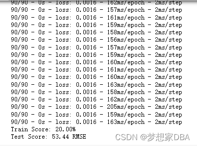
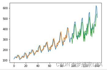
plt.show()Running the model produces the following output.
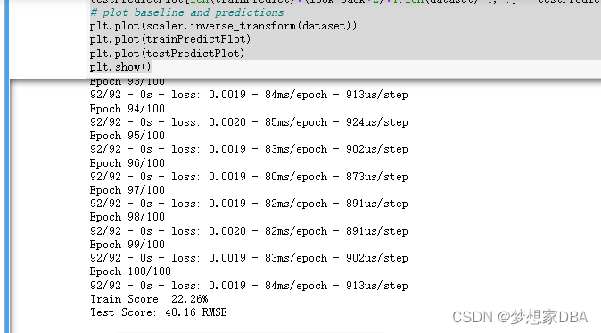
We can see that the model did an OK job of fitting both the training and the test datasets.
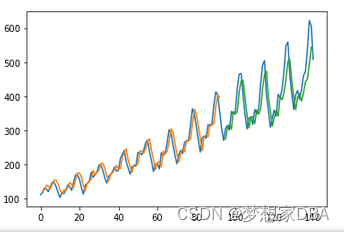
We can see that the model has an average error of about 23 passengers (in thousands) on the training dataset and about 52 passengers (in thousands) on the test dataset. Not that bad.
1.2 LSTM For Regression Using the Window Method
We can also phrase the problem so that multiple recent time steps can be used to make the prediction for the next time step. This is called a window and the size of the window is a parameter that can be tuned for each problem. For example, given the current time (t) we want to predict the value at the next time in the sequence (t+1), we can use the current time (t) as well as the two prior times (t-1 and t-2) as input variables. When phrased as a regression problem the input variables are t-2, t-1, t and the output variable is t+1.
The create_dataset() function we created in the previous section allows us to create this formulation of the time series problem by increasing the look back argument from 1 to 3. A sample of the dataset with this formulation looks as follows:
X1 X2 X3 Y
112 118 132 129
118 132 129 121
132 129 121 135
129 121 135 148
121 135 148 148
We can re-run the example in the previous section with the larger window size. The whole code listing with just the window size change is listed below for completeness.
# LSTM for international airline passengers problem with regression framing
import numpy as np
import matplotlib.pyplot as plt
import pandas as pd
import math
from keras.models import Sequential
from keras.layers import Dense
from keras.layers import LSTM
from sklearn.preprocessing import MinMaxScaler
from sklearn.metrics import mean_squared_error
# convert an array of values into a dataset matrix
def create_dataset(dataset, look_back=1):
dataX, dataY = [],[]
for i in range(len(dataset)-look_back-1):
a = dataset[i:(i+look_back),0]
dataX.append(a)
dataY.append(dataset[i + look_back,0])
return np.array(dataX), np.array(dataY)
# fix random seed for reproducibility
seed = 7
np.random.seed(seed)
# load the dataset
dataframe = pd.read_csv('international-airline-passengers.csv',usecols=[1],engine='python',skipfooter=3)
dataset = dataframe.values
dataset = dataset.astype('float32')
# normalize the dataset
scaler = MinMaxScaler(feature_range=(0, 1))
dataset = scaler.fit_transform(dataset)
# split into train and test sets
train_size = int(len(dataset) * 0.67)
test_size = len(dataset) - train_size
train, test = dataset[0:train_size,:],dataset[train_size:len(dataset),:]
# reshape into X=t and Y=t+1
look_back = 3
trainX, trainY = create_dataset(train, look_back)
testX, testY = create_dataset(test, look_back)
# reshape input to be [samples, time steps, features]
trainX = np.reshape(trainX,(trainX.shape[0], 1, trainX.shape[1]))
testX = np.reshape(testX, (testX.shape[0], 1, testX.shape[1]))
# create and fit the LSTM network
model = Sequential()
model.add(LSTM(4, input_dim=look_back))
model.add(Dense(1))
model.compile(loss='mean_squared_error',optimizer='adam')
model.fit(trainX,trainY,epochs=100, batch_size=1,verbose=2)
# make predictions
trainPredict = model.predict(trainX)
testPredict = model.predict(testX)
#invert predictions
trainPredict = scaler.inverse_transform(trainPredict)
trainY = scaler.inverse_transform([trainY])
testPredict = scaler.inverse_transform(testPredict)
testY = scaler.inverse_transform([testY])
# calculate root mean suqared error
trainScore = math.sqrt(mean_squared_error(trainY[0],trainPredict[:,0]))
print('Train Score: %.2f%%'% (trainScore))
testScore = math.sqrt(mean_squared_error(testY[0],testPredict[:,0]))
print('Test Score: %.2f RMSE' %(testScore))
#shift train prediction for plotting
trainPredictPlot = np.empty_like(dataset)
trainPredictPlot[:, :] = np.nan
trainPredictPlot[look_back:len(trainPredict)+look_back,:] = trainPredict
# shift test predictions for plotting
testPredictPlot = np.empty_like(dataset)
testPredictPlot[:, :] = np.nan
testPredictPlot[len(trainPredict)+(look_back*2)+1:len(dataset)-1, :] = testPredict
# plot baseline and predictions
plt.plot(scaler.inverse_transform(dataset))
plt.plot(trainPredictPlot)
plt.plot(testPredictPlot)
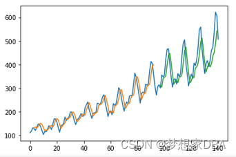
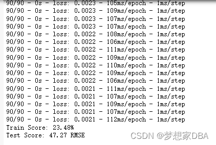
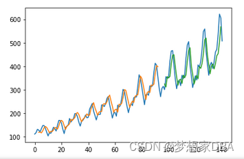
plt.show()Running the example provides the following output.
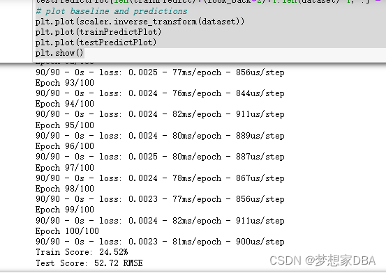
We can see that the error was increased slightly compared to that of the previous section. The window size and the network architecture were not tuned, this is just a demonstration of how to frame a prediction problem.
1.3 LSTM For Regression with Time Steps
You may have noticed that the data preparation for the LSTM network includes time steps. Some sequence problems may have a varied number of time steps per sample. For example, you may have measurements of a physical machine leading up to a point of failure or a point of surge. Each incident would be a sample, the observations that lead up to the event would be the time steps and the variables observed would be the features. Time steps provides another way to phrase our time series problem. Like above in the window example, we can take prior time steps in our time series as inputs to predict the output at the next time step.
Instead of phrasing the past observations as separate input features, we can use them as time steps of the one input feature, which is indeed a more accurate framing of the problem.
We can do this using the same data representation as in the previous window-based example, except when we reshape the data we set the columns to be the time steps dimension and change the features dimension back to 1. For example:
# reshape input to be [samples, time steps, features]
trainX = numpy.reshape(trainX, (trainX.shape[0], trainX.shape[1], 1))
testX = numpy.reshape(testX, (testX.shape[0], testX.shape[1], 1))
The entire code listing is provided below for completeness.
# LSTM for international airline passengers problem with time step regression framing
import numpy as np
import matplotlib.pyplot as plt
import pandas as pd
import math
from keras.models import Sequential
from keras.layers import Dense
from keras.layers import LSTM
from sklearn.preprocessing import MinMaxScaler
from sklearn.metrics import mean_squared_error

# convert an array of values into a dataset matrix
def create_dataset(dataset, look_back=1):
    dataX, dataY = [],[]
    for i in range(len(dataset)-look_back-1):
        a = dataset[i:(i+look_back),0]
        dataX.append(a)
        dataY.append(dataset[i + look_back,0])
    return np.array(dataX), np.array(dataY)

# fix random seed for reproducibility
seed = 7
np.random.seed(seed)

# load the dataset
dataframe = pd.read_csv('international-airline-passengers.csv',usecols=[1],engine='python',skipfooter=3)
dataset = dataframe.values
dataset = dataset.astype('float32')

# normalize the dataset
scaler = MinMaxScaler(feature_range=(0, 1))
dataset = scaler.fit_transform(dataset)

# split into train and test sets
train_size = int(len(dataset) * 0.67)
test_size = len(dataset) - train_size
train, test = dataset[0:train_size,:],dataset[train_size:len(dataset),:]

# reshape into X=t and Y=t+1
look_back = 3
trainX, trainY = create_dataset(train, look_back)
testX, testY = create_dataset(test, look_back)

# reshape input to be [samples, time steps, features]
trainX = np.reshape(trainX,(trainX.shape[0], trainX.shape[1], 1))
testX = np.reshape(testX, (testX.shape[0], testX.shape[1], 1))
# create and fit the LSTM network
model = Sequential()
model.add(LSTM(4, input_dim=1))
model.add(Dense(1))
model.compile(loss='mean_squared_error',optimizer='adam')
model.fit(trainX,trainY,epochs=100, batch_size=1,verbose=2)
# make predictions
trainPredict = model.predict(trainX)
testPredict = model.predict(testX)
#invert predictions
trainPredict = scaler.inverse_transform(trainPredict)
trainY = scaler.inverse_transform([trainY])
testPredict = scaler.inverse_transform(testPredict)
testY = scaler.inverse_transform([testY])

# calculate root mean suqared error
trainScore = math.sqrt(mean_squared_error(trainY[0],trainPredict[:,0]))
print('Train Score: %.2f%%'% (trainScore))
testScore = math.sqrt(mean_squared_error(testY[0],testPredict[:,0]))
print('Test Score: %.2f RMSE' %(testScore))

#shift train prediction for plotting
trainPredictPlot = np.empty_like(dataset)
trainPredictPlot[:, :] = np.nan
trainPredictPlot[look_back:len(trainPredict)+look_back,:] = trainPredict

# shift test predictions for plotting
testPredictPlot = np.empty_like(dataset)
testPredictPlot[:, :] = np.nan
testPredictPlot[len(trainPredict)+(look_back*2)+1:len(dataset)-1, :] = testPredict
# plot baseline and predictions
plt.plot(scaler.inverse_transform(dataset))
plt.plot(trainPredictPlot)
plt.plot(testPredictPlot)
plt.show()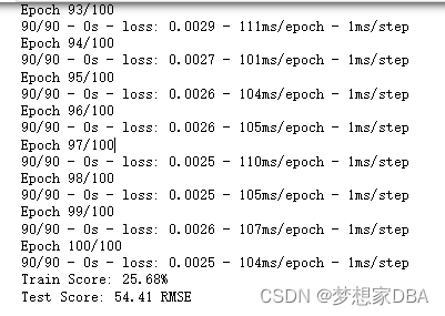
We can see that the error was increased slightly compared to that of the previous section. The window size and the network architecture were not tuned, this is just a demonstration of how to frame a prediction problem.
1.4 LSTM With Memory Between Batches
The LSTM network has memory which is capable of remembering across long sequences. Normally, the state within the network is reset after each training batch when fitting the model, as well as each call to model.predict() or model.evaluate(). We can gain finer control over when the internal state of the LSTM network is cleared in Keras by making the LSTM layer stateful. This means that it can build state over the entire training sequence and even maintain that state if needed to make predictions. It requires that the training data not be shu✏ed when fitting the network. It also requires explicit resetting of the network state after each exposure to the training data (epoch) by calls to model.reset states(). This means that we must create our own outer loop of epochs and within each epoch call model.fit() and model.reset states(), for example:
for i in range(100):
    model.fit(trainX, trainY,epochs=1,batch_size=batch_size,verbose=2,shuffle=False)
    model.rest_states()
Finally, when the LSTM layer is constructed, the stateful parameter must be set to True and instead of specifying the input dimensions, we must hard code the number of samples in a batch, number of time steps in a sample and number of features in a time step by setting the batch input shape parameter. For example:
model.add(LSTM(4, batch_input_shape=(batch_size, time_steps, features), stateful=True))This same batch size must then be used later when evaluating the model and making predictions. For example:
model.predict(trainX, batch_size=batch_size)We can adapt the previous time step example to use a stateful LSTM. The full code listing is provided below.
# LSTM for international airline passengers problem with time step regression framing
import numpy as np
import matplotlib.pyplot as plt
import pandas as pd
import math
from keras.models import Sequential
from keras.layers import Dense
from keras.layers import LSTM
from sklearn.preprocessing import MinMaxScaler
from sklearn.metrics import mean_squared_error

# convert an array of values into a dataset matrix
def create_dataset(dataset, look_back=1):
    dataX, dataY = [],[]
    for i in range(len(dataset)-look_back-1):
        a = dataset[i:(i+look_back),0]
        dataX.append(a)
        dataY.append(dataset[i + look_back,0])
    return np.array(dataX), np.array(dataY)

# fix random seed for reproducibility
seed = 7
np.random.seed(seed)

# load the dataset
dataframe = pd.read_csv('international-airline-passengers.csv',usecols=[1],engine='python',skipfooter=3)
dataset = dataframe.values
dataset = dataset.astype('float32')

# normalize the dataset
scaler = MinMaxScaler(feature_range=(0, 1))
dataset = scaler.fit_transform(dataset)

# split into train and test sets
train_size = int(len(dataset) * 0.67)
test_size = len(dataset) - train_size
train, test = dataset[0:train_size,:],dataset[train_size:len(dataset),:]

# reshape into X=t and Y=t+1
look_back = 3
trainX, trainY = create_dataset(train, look_back)
testX, testY = create_dataset(test, look_back)

# reshape input to be [samples, time steps, features]
trainX = np.reshape(trainX,(trainX.shape[0], trainX.shape[1], 1))
testX = np.reshape(testX, (testX.shape[0], testX.shape[1], 1))

# create and fit the LSTM network
batch_size = 1
model = Sequential()
model.add(LSTM(4, batch_input_shape=(batch_size,look_back,1),stateful=True))
model.add(Dense(1))
model.compile(loss='mean_squared_error',optimizer='adam')
for i in range(100):
    model.fit(trainX,trainY,epochs=1, batch_size=batch_size,verbose=2,shuffle=False)
    model.reset_states()
# make predictions
trainPredict = model.predict(trainX, batch_size=batch_size)
testPredict = model.predict(testX, batch_size=batch_size)
#invert predictions
trainPredict = scaler.inverse_transform(trainPredict)
trainY = scaler.inverse_transform([trainY])
testPredict = scaler.inverse_transform(testPredict)
testY = scaler.inverse_transform([testY])

# calculate root mean suqared error
trainScore = math.sqrt(mean_squared_error(trainY[0],trainPredict[:,0]))
print('Train Score: %.2f%%'% (trainScore))
testScore = math.sqrt(mean_squared_error(testY[0],testPredict[:,0]))
print('Test Score: %.2f RMSE' %(testScore))

#shift train prediction for plotting
trainPredictPlot = np.empty_like(dataset)
trainPredictPlot[:, :] = np.nan
trainPredictPlot[look_back:len(trainPredict)+look_back,:] = trainPredict

# shift test predictions for plotting
testPredictPlot = np.empty_like(dataset)
testPredictPlot[:, :] = np.nan
testPredictPlot[len(trainPredict)+(look_back*2)+1:len(dataset)-1, :] = testPredict
# plot baseline and predictions
plt.plot(scaler.inverse_transform(dataset))
plt.plot(trainPredictPlot)
plt.plot(testPredictPlot)
plt.show()
Running the example provides the following output:
We do see that results are worse. The model may need more modules and may need to be trained for more epochs to internalize the structure of thee problem.
1.5 Stacked LSTMs With Memory Between Batches
Finally, we will take a look at one of the big benefits of LSTMs, the fact that they can be successfully trained when stacked into deep network architectures. LSTM networks can be stacked in Keras in the same way that other layer types can be stacked. One addition to the configuration that is required is that an LSTM layer prior to each subsequent LSTM layer must return the sequence. This can be done by setting the return sequences parameter on the layer to True. We can extend the stateful LSTM in the previous section to have two layers, as follows:
model.add(LSTM(4, batch_input_shape=(batch_size, look_back, 1), stateful=True,
return_sequences=True))
model.add(LSTM(4, batch_input_shape=(batch_size, look_back, 1), stateful=True))
The entire code listing is provided below for completeness.
# Stacked LSTM for international airline passengers problem with memory
import numpy as np
import matplotlib.pyplot as plt
import pandas as pd
import math
from keras.models import Sequential
from keras.layers import Dense
from keras.layers import LSTM
from sklearn.preprocessing import MinMaxScaler
from sklearn.metrics import mean_squared_error

# convert an array of values into a dataset matrix
def create_dataset(dataset, look_back=1):
    dataX, dataY = [],[]
    for i in range(len(dataset)-look_back-1):
        a = dataset[i:(i+look_back),0]
        dataX.append(a)
        dataY.append(dataset[i + look_back,0])
    return np.array(dataX), np.array(dataY)

# fix random seed for reproducibility
seed = 7
np.random.seed(seed)

# load the dataset
dataframe = pd.read_csv('international-airline-passengers.csv',usecols=[1],engine='python',skipfooter=3)
dataset = dataframe.values
dataset = dataset.astype('float32')

# normalize the dataset
scaler = MinMaxScaler(feature_range=(0, 1))
dataset = scaler.fit_transform(dataset)

# split into train and test sets
train_size = int(len(dataset) * 0.67)
test_size = len(dataset) - train_size
train, test = dataset[0:train_size,:],dataset[train_size:len(dataset),:]

# reshape into X=t and Y=t+1
look_back = 3
trainX, trainY = create_dataset(train, look_back)
testX, testY = create_dataset(test, look_back)

# reshape input to be [samples, time steps, features]
trainX = np.reshape(trainX,(trainX.shape[0], trainX.shape[1], 1))
testX = np.reshape(testX, (testX.shape[0], testX.shape[1], 1))

# create and fit the LSTM network
batch_size = 1
model = Sequential()
model.add(LSTM(4, batch_input_shape=(batch_size,look_back,1),stateful=True,return_sequences=True))
model.add(LSTM(4, batch_input_shape=(batch_size,look_back,1),stateful=True))
model.add(Dense(1))
model.compile(loss='mean_squared_error',optimizer='adam')
for i in range(100):
    model.fit(trainX,trainY,epochs=1, batch_size=batch_size,verbose=2,shuffle=False)
    model.reset_states()
# make predictions
trainPredict = model.predict(trainX, batch_size=batch_size)
model.reset_states()
testPredict = model.predict(testX, batch_size=batch_size)
#invert predictions
trainPredict = scaler.inverse_transform(trainPredict)
trainY = scaler.inverse_transform([trainY])
testPredict = scaler.inverse_transform(testPredict)
testY = scaler.inverse_transform([testY])

# calculate root mean suqared error
trainScore = math.sqrt(mean_squared_error(trainY[0],trainPredict[:,0]))
print('Train Score: %.2f%%'% (trainScore))
testScore = math.sqrt(mean_squared_error(testY[0],testPredict[:,0]))
print('Test Score: %.2f RMSE' %(testScore))

#shift train prediction for plotting
trainPredictPlot = np.empty_like(dataset)
trainPredictPlot[:, :] = np.nan
trainPredictPlot[look_back:len(trainPredict)+look_back,:] = trainPredict

# shift test predictions for plotting
testPredictPlot = np.empty_like(dataset)
testPredictPlot[:, :] = np.nan
testPredictPlot[len(trainPredict)+(look_back*2)+1:len(dataset)-1, :] = testPredict
# plot baseline and predictions
plt.plot(scaler.inverse_transform(dataset))
plt.plot(trainPredictPlot)
plt.plot(testPredictPlot)
plt.show()
Running the example produces the following output.
The predictions on the test dataset are again worse. This is more evidence to suggest the need for additional training epochs.
1.6 Summary
In this lesson you discovered how to develop LSTM recurrent neural networks for time series prediction in Python with the Keras deep learning network. Specifically, you learned:
About the international airline passenger time series prediction problem.
- How to create an LSTM for a regression and a window formulation of the time series problem.
- How to create an LSTM with a time step formulation of the time series problem.
- How to create an LSTM with state and stacked LSTMs with state to learn long sequences.


 被折叠的 条评论
为什么被折叠?
被折叠的 条评论
为什么被折叠?
 到【灌水乐园】发言


