


Part 2
第二部分的理解,将会着力于如何使用tensorflow的扫描和动态rnn模型,把RNN单元升级到多RNN堆叠的形式,并且
增加dropout和正则化。然后使用升级版的RNN来产生文字。
任务和数据
这次我们要建立一个字符级的语言模型来产生字符序列。 char-rnn (tensorflow中有开源实现)。这次的任务比上次难很多。
这个模型需要解决长序列和学习长时依赖性,对我们给RNN增加特征填了很多麻烦,看我们的改变是如何影响到结果的。
首先,让我们创建一个数据的产生器,把小型莎士比亚文集作为我们的数据,其他任何文本也都可以。然后把文本里所有
的字符都作为我们的词汇,把小写和大写字母当作单独的字符处理。实际上,如果强制网络用相似的表示方法来处理大小
写字母,比如用one-hot表示法,并且最后增加一个大小写位,这样可能会更好。另外,如果把一些不常见的字母用UNK来
代替,也可以起到限制词汇量的作用,这也是一个不错的主意。
"""
Imports
"""
import numpy as np
import tensorflow as tf
import matplotlib.pyplot as plt
import time
import os
import urllib.request
from tensorflow.models.rnn.ptb import reader
"""
Load and process data, utility functions
"""
file_url = 'https://raw.githubusercontent.com/jcjohnson/torch-rnn/master/data/tiny-shakespeare.txt'
file_name = 'tinyshakespeare.txt'
if not os.path.exists(file_name):
urllib.request.urlretrieve(file_url, file_name)
with open(file_name,'r') as f:
raw_data = f.read()
print("Data length:", len(raw_data))
vocab = set(raw_data)
vocab_size = len(vocab)
idx_to_vocab = dict(enumerate(vocab))
vocab_to_idx = dict(zip(idx_to_vocab.values(), idx_to_vocab.keys()))
data = [vocab_to_idx[c] for c in raw_data]
del raw_data
def gen_epochs(n, num_steps, batch_size):
for i in range(n):
yield reader.ptb_iterator(data, batch_size, num_steps)
def reset_graph():
if 'sess' in globals() and sess:
sess.close()
tf.reset_default_graph()
def train_network(g, num_epochs, num_steps = 200, batch_size = 32, verbose = True, save=False):
tf.set_random_seed(2345)
with tf.Session() as sess:
sess.run(tf.initialize_all_variables())
training_losses = []
for idx, epoch in enumerate(gen_epochs(num_epochs, num_steps, batch_size)):
training_loss = 0
steps = 0
training_state = None
for X, Y in epoch:
steps += 1
feed_dict={g['x']: X, g['y']: Y}
if training_state is not None:
feed_dict[g['init_state']] = training_state
training_loss_, training_state, _ = sess.run([g['total_loss'],
g['final_state'],
g['train_step']],
feed_dict)
training_loss += training_loss_
if verbose:
print("Average training loss for Epoch", idx, ":", training_loss/steps)
training_losses.append(training_loss/steps)
if isinstance(save, str):
g['saver'].save(sess, save)
return training_lossesData length: 1115394利用tf.scan和dynamicRNN来加速训练
回忆一下上一篇里我们把每个重复的RNN张量表示成张量列表;
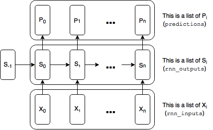
这个非常有效,因为我们最长的依赖在7步之前,不必把误差回传超过10步。即便是单词级别的RNN,使用列表也可能是
有效的。之前一篇博客里用了截断反向传播,建立了一个40步的图都没有问题,但是对一个字符级别的模型,40个字符
远远不够,我们想要捕获更长期的依赖。来看一下构造200步宽的图会发生什么事情。
def build_basic_rnn_graph_with_list(
    state_size = 100,
    num_classes = vocab_size,
    batch_size = 32,
    num_steps = 200,
    learning_rate = 1e-4):

    reset_graph()

    x = tf.placeholder(tf.int32, [batch_size, num_steps], name='input_placeholder')
    y = tf.placeholder(tf.int32, [batch_size, num_steps], name='labels_placeholder')

    x_one_hot = tf.one_hot(x, num_classes)
    rnn_inputs = [tf.squeeze(i,squeeze_dims=[1]) for i in tf.split(1, num_steps, x_one_hot)]

    cell = tf.nn.rnn_cell.BasicRNNCell(state_size)
    init_state = cell.zero_state(batch_size, tf.float32)
    rnn_outputs, final_state = tf.nn.rnn(cell, rnn_inputs, initial_state=init_state)

    with tf.variable_scope('softmax'):
        W = tf.get_variable('W', [state_size, num_classes])
        b = tf.get_variable('b', [num_classes], initializer=tf.constant_initializer(0.0))
    logits = [tf.matmul(rnn_output, W) + b for rnn_output in rnn_outputs]

    y_as_list = [tf.squeeze(i, squeeze_dims=[1]) for i in tf.split(1, num_steps, y)]

    loss_weights = [tf.ones([batch_size]) for i in range(num_steps)]
    losses = tf.nn.seq2seq.sequence_loss_by_example(logits, y_as_list, loss_weights)
    total_loss = tf.reduce_mean(losses)
    train_step = tf.train.AdamOptimizer(learning_rate).minimize(total_loss)

    return dict(
        x = x,
        y = y,
        init_state = init_state,
        final_state = final_state,
        total_loss = total_loss,
        train_step = train_step
    )
t = time.time()
build_basic_rnn_graph_with_list()
print("It took", time.time() - t, "seconds to build the graph.")It took 5.626644849777222 seconds to build the graph.def build_multilayer_lstm_graph_with_list(
state_size = 100,
num_classes = vocab_size,
batch_size = 32,
num_steps = 200,
num_layers = 3,
learning_rate = 1e-4):
reset_graph()
x = tf.placeholder(tf.int32, [batch_size, num_steps], name='input_placeholder')
y = tf.placeholder(tf.int32, [batch_size, num_steps], name='labels_placeholder')
embeddings = tf.get_variable('embedding_matrix', [num_classes, state_size])
rnn_inputs = [tf.squeeze(i) for i in tf.split(1,
num_steps, tf.nn.embedding_lookup(embeddings, x))]
cell = tf.nn.rnn_cell.LSTMCell(state_size, state_is_tuple=True)
cell = tf.nn.rnn_cell.MultiRNNCell([cell] * num_layers, state_is_tuple=True)
init_state = cell.zero_state(batch_size, tf.float32)
rnn_outputs, final_state = tf.nn.rnn(cell, rnn_inputs, initial_state=init_state)
with tf.variable_scope('softmax'):
W = tf.get_variable('W', [state_size, num_classes])
b = tf.get_variable('b', [num_classes], initializer=tf.constant_initializer(0.0))
logits = [tf.matmul(rnn_output, W) + b for rnn_output in rnn_outputs]
y_as_list = [tf.squeeze(i, squeeze_dims=[1]) for i in tf.split(1, num_steps, y)]
loss_weights = [tf.ones([batch_size]) for i in range(num_steps)]
losses = tf.nn.seq2seq.sequence_loss_by_example(logits, y_as_list, loss_weights)
total_loss = tf.reduce_mean(losses)
train_step = tf.train.AdamOptimizer(learning_rate).minimize(total_loss)
return dict(
x = x,
y = y,
init_state = init_state,
final_state = final_state,
total_loss = total_loss,
train_step = train_step
)t = time.time()
build_multilayer_lstm_graph_with_list()
print("It took", time.time() - t, "seconds to build the graph.")It took 25.640846967697144 seconds to build the graph.
虽然对训练的问题不是很大,因为构图只需要一次,但是我们要在测试的时候构造好几次图。为了解决这个问题,tensorflow允许我们
在运行的时候构造图。下面是一个例子,利用的动态rnn函数。
def build_multilayer_lstm_graph_with_dynamic_rnn(
    state_size = 100,
    num_classes = vocab_size,
    batch_size = 32,
    num_steps = 200,
    num_layers = 3,
    learning_rate = 1e-4):

    reset_graph()

    x = tf.placeholder(tf.int32, [batch_size, num_steps], name='input_placeholder')
    y = tf.placeholder(tf.int32, [batch_size, num_steps], name='labels_placeholder')

    embeddings = tf.get_variable('embedding_matrix', [num_classes, state_size])

    # Note that our inputs are no longer a list, but a tensor of dims batch_size x num_steps x state_size
    rnn_inputs = tf.nn.embedding_lookup(embeddings, x)

    cell = tf.nn.rnn_cell.LSTMCell(state_size, state_is_tuple=True)
    cell = tf.nn.rnn_cell.MultiRNNCell([cell] * num_layers, state_is_tuple=True)
    init_state = cell.zero_state(batch_size, tf.float32)
    rnn_outputs, final_state = tf.nn.dynamic_rnn(cell, rnn_inputs, initial_state=init_state)

    with tf.variable_scope('softmax'):
        W = tf.get_variable('W', [state_size, num_classes])
        b = tf.get_variable('b', [num_classes], initializer=tf.constant_initializer(0.0))

    #reshape rnn_outputs and y so we can get the logits in a single matmul
    rnn_outputs = tf.reshape(rnn_outputs, [-1, state_size])
    y_reshaped = tf.reshape(y, [-1])

    logits = tf.matmul(rnn_outputs, W) + b

    total_loss = tf.reduce_mean(tf.nn.sparse_softmax_cross_entropy_with_logits(logits, y_reshaped))
    train_step = tf.train.AdamOptimizer(learning_rate).minimize(total_loss)

    return dict(
        x = x,
        y = y,
        init_state = init_state,
        final_state = final_state,
        total_loss = total_loss,
        train_step = train_step
    )
t = time.time()
build_multilayer_lstm_graph_with_dynamic_rnn()
print("It took", time.time() - t, "seconds to build the graph.")It took 0.5314393043518066 seconds to build the graph.快了很多!可能有人会认为把构图操作放在执行阶段会拖慢执行的速度,但实际上,动态RNN确实加快了速度。
g = build_multilayer_lstm_graph_with_list()
t = time.time()
train_network(g, 3)
print("It took", time.time() - t, "seconds to train for 3 epochs.")
Average training loss for Epoch 0 : 3.53323210245
Average training loss for Epoch 1 : 3.31435756163
Average training loss for Epoch 2 : 3.21755325109
It took 117.78161263465881 seconds to train for 3 epochs.g = build_multilayer_lstm_graph_with_dynamic_rnn()
t = time.time()
train_network(g, 3)
print("It took", time.time() - t, "seconds to train for 3 epochs.")Average training loss for Epoch 0 : 3.55792756053
Average training loss for Epoch 1 : 3.3225021006
Average training loss for Epoch 2 : 3.28286816745
It took 96.69413661956787 seconds to train for 3 epochs.可能彻底理解动态RNN的代码并不是那么容易的事情,但我们可以用tf.scan来实现类似的功能(动态rnn没有使用scan).
scan只比tensorflow优化代码慢一点点,但是非常容易理解和实现。这里先不实现这部分内容。
升级RNN单元
上面,我们无缝的把BasicRNNCell包裹成我们用的多层LSTM单元,这可能是因为RNN单元符合一个通用的结构:每一个RNN单元是
一个当前的输入Xt,和前一步的状态St-1,然后输出当前的状态St和当前的输出Yt.因此,以同样的方法可以在前向传播时包裹激活函数,
我们甚至可以包裹整个循环神经网络。
需要注意的是,基础的RNN单元他们的当前输出等于当前的状态(Yt=St),但并不总是如此。看一下LSTMs和多层RNN是如何变化的。
RNN单元两个常用的选择是GRU和LSTM。通过引入门的概念,GRU和LSTM避免了梯度消失问题,并且允许网络可以学习到更长期
的独立性。他们的内部非常负责,可以另起一篇文章来讲述他们。
我们在本文中要做的就是把RNN单元升级一下。
cell = tf.nn.rnn_cell.BasicRNNCell(state_size)cell = tf.nn.rnn_cell.LSTMCell(state_size)cell = tf.nn.rnn_cell.GRUCell(state_size)LSTM存储了两个内部状态向量,c和h, c是记忆单元或者常数错误,h是隐藏状态。默认情况下,他们被连接成一个单独的向量,但是
会出现下面的警告信息:
WARNING:tensorflow:<tensorflow.python.ops.rnn_cell.LSTMCell object at 0x7faade1708d0>: Using a concatenated state is slower and will soon be deprecated. Use state_is_tuple=True.这个错误告诉我们的是用一个c和h的元组来表示LSTM的状态会比c和h的连接形式更好,你可以用参数state_is_tuple=True来切换。
通过元组的状态形式,我们也可以非常轻松的把MultiyRNNCell表示层多层。可以通过下图想明白其中的原因:

可以看一下两个单元堆叠之后在的不同之处
可以看一下两个单元堆叠之后在的不同之处

之后,我们可以把两个单元包裹起来,使他们看上去像一个单一的单元。

要做到这一点,我们调用tf.nn.rnn_cell.MultiRNNCell,它把一个list的RNNCells作为输入
并且把他们包裹成一个单一的cell:
cell = tf.nn.rnn_cell.MultiRNNCell([tf.nn.rnn_cell.BasicRNNCell(state_size)] * num_layers)写一个定制版的RNN cell
如果仅仅使用标准的GRU和LSTM单元,那是实在太容易了,所以让我们来定义一个自己的RNN单元。
这是一个比较草率的想法,并且可能不奏效:启动一个GRU单元,对输入进行多次变换而不是做一些
简单变换。利用Cho et al.(2014)文中的记法,我们对输入W1x,W2x,W3x...Wnx进行加权,用
ΣλiWix
取代
Wx , λi 的和为1. 这个新的权重λ 将会被计算成:λ=softmax(Wavgx(t)+Uavgh(t−1)+b) 。
这个想法就是如果对输入进行多层变换,可能会得到一些不错的功效,例如我们可能对名词和动词会有
不同的处理方法。
为了写出这个定制单元的代码,我们需要拓展tf.nn.rnn_cell.RNNCell. 特别地,我们需要实现三个抽象方法,
然后写一个__init__初始化方法(可以看一下tensorflow代码).
首先,让我们从GRU开始定制。
class GRUCell(tf.nn.rnn_cell.RNNCell):
    """Gated Recurrent Unit cell (cf. http://arxiv.org/abs/1406.1078)."""

    def __init__(self, num_units):
        self._num_units = num_units

    @property
    def state_size(self):
        return self._num_units

    @property
    def output_size(self):
        return self._num_units

    def __call__(self, inputs, state, scope=None):
        with tf.variable_scope(scope or type(self).__name__):  # "GRUCell"
            with tf.variable_scope("Gates"):  # Reset gate and update gate.
                # We start with bias of 1.0 to not reset and not update.
                ru = tf.nn.rnn_cell._linear([inputs, state],
                                        2 * self._num_units, True, 1.0)
                ru = tf.nn.sigmoid(ru)
                r, u = tf.split(1, 2, ru)
            with tf.variable_scope("Candidate"):
                c = tf.nn.tanh(tf.nn.rnn_cell._linear([inputs, r * state],
                                             self._num_units, True))
            new_h = u * state + (1 - u) * c
return new_h, new_hdef __init__(self, num_units, num_weights):
self._num_units = num_units
self._num_weights = num_weights然后,修改__call__方法里Candidate的变量scope,来做一个平均加权,注意所有的Wi矩阵
作为一个单独的变量被创建然后分成许多张量。
class CustomCell(tf.nn.rnn_cell.RNNCell):
"""Gated Recurrent Unit cell (cf. http://arxiv.org/abs/1406.1078)."""
def __init__(self, num_units, num_weights):
    self._num_units = num_units
    self._num_weights = num_weights
@property
def state_size(self):
return self._num_units
@property
def output_size(self):
return self._num_units
def __call__(self, inputs, state, scope=None):
with tf.variable_scope(scope or type(self).__name__): # "GRUCell"
with tf.variable_scope("Gates"): # Reset gate and update gate.
# We start with bias of 1.0 to not reset and not update.
ru = tf.nn.rnn_cell._linear([inputs, state],
2 * self._num_units, True, 1.0)
ru = tf.nn.sigmoid(ru)
r, u = tf.split(1, 2, ru)
with tf.variable_scope("Candidate"):
lambdas = tf.nn.rnn_cell._linear([inputs, state], self._num_weights, True)
lambdas = tf.split(1, self._num_weights, tf.nn.softmax(lambdas))
Ws = tf.get_variable("Ws",
shape = [self._num_weights, inputs.get_shape()[1], self._num_units])
Ws = [tf.squeeze(i) for i in tf.split(0, self._num_weights, Ws)]
candidate_inputs = []
for idx, W in enumerate(Ws):
candidate_inputs.append(tf.matmul(inputs, W) * lambdas[idx])
Wx = tf.add_n(candidate_inputs)
c = tf.nn.tanh(Wx + tf.nn.rnn_cell._linear([r * state],
self._num_units, True, scope="second"))
new_h = u * state + (1 - u) * c
return new_h, new_hdef build_multilayer_graph_with_custom_cell(
cell_type = None,
num_weights_for_custom_cell = 5,
state_size = 100,
num_classes = vocab_size,
batch_size = 32,
num_steps = 200,
num_layers = 3,
learning_rate = 1e-4):
reset_graph()
x = tf.placeholder(tf.int32, [batch_size, num_steps], name='input_placeholder')
y = tf.placeholder(tf.int32, [batch_size, num_steps], name='labels_placeholder')
embeddings = tf.get_variable('embedding_matrix', [num_classes, state_size])
rnn_inputs = tf.nn.embedding_lookup(embeddings, x)
if cell_type == 'Custom':
cell = CustomCell(state_size, num_weights_for_custom_cell)
elif cell_type == 'GRU':
cell = tf.nn.rnn_cell.GRUCell(state_size)
elif cell_type == 'LSTM':
cell = tf.nn.rnn_cell.LSTMCell(state_size, state_is_tuple=True)
else:
cell = tf.nn.rnn_cell.BasicRNNCell(state_size)
if cell_type == 'LSTM':
cell = tf.nn.rnn_cell.MultiRNNCell([cell] * num_layers, state_is_tuple=True)
else:
cell = tf.nn.rnn_cell.MultiRNNCell([cell] * num_layers)
init_state = cell.zero_state(batch_size, tf.float32)
rnn_outputs, final_state = tf.nn.dynamic_rnn(cell, rnn_inputs, initial_state=init_state)
with tf.variable_scope('softmax'):
W = tf.get_variable('W', [state_size, num_classes])
b = tf.get_variable('b', [num_classes], initializer=tf.constant_initializer(0.0))
#reshape rnn_outputs and y
rnn_outputs = tf.reshape(rnn_outputs, [-1, state_size])
y_reshaped = tf.reshape(y, [-1])
logits = tf.matmul(rnn_outputs, W) + b
total_loss = tf.reduce_mean(tf.nn.sparse_softmax_cross_entropy_with_logits(logits, y_reshaped))
train_step = tf.train.AdamOptimizer(learning_rate).minimize(total_loss)
return dict(
x = x,
y = y,
init_state = init_state,
final_state = final_state,
total_loss = total_loss,
train_step = train_step
)
g = build_multilayer_graph_with_custom_cell(cell_type='GRU', num_steps=30)
t = time.time()
train_network(g, 5, num_steps=30)
print("It took", time.time() - t, "seconds to train for 5 epochs.")
Average training loss for Epoch 0 : 2.92919953048
Average training loss for Epoch 1 : 2.35888109404
Average training loss for Epoch 2 : 2.21945820894
Average training loss for Epoch 3 : 2.12258511006
Average training loss for Epoch 4 : 2.05038544733
It took 284.6971204280853 seconds to train for 5 epochs.g = build_multilayer_graph_with_custom_cell(cell_type='Custom', num_steps=30)
t = time.time()
train_network(g, 5, num_steps=30)
print("It took", time.time() - t, "seconds to train for 5 epochs.")Average training loss for Epoch 0 : 3.04418995892
Average training loss for Epoch 1 : 2.5172702761
Average training loss for Epoch 2 : 2.37068433601
Average training loss for Epoch 3 : 2.27533404217
Average training loss for Epoch 4 : 2.20167231745
It took 537.6112766265869 seconds to train for 5 epochs.由于起初的方法,我们的定制单元花了两倍多的时间,似乎比标准的GRU表现不如。
增加Dropout
给网络增加dropout并不难,我们解决在哪里加进去的问题。
Dropout属于层间,不属于状态或者内部单元的连接部分。看一下
Zaremba et al. (2015),
Recurrent Neural Network Regularization, 想法就是只在非递归的部分增加dropout操作。
因此,我们需要包裹一下每个单元的输入或者输出以便增加dropout. 在我们的RNN实现中
使用了list,我们会做一些类似的事情:
rnn_inputs = [tf.nn.dropout(rnn_input, keep_prob) for rnn_input in rnn_inputs]
rnn_outputs = [tf.nn.dropout(rnn_output, keep_prob) for nn_output in rnn_outputs]
答案是把基本RNN单元用dropout封装,因此可以类似于我们把3个RNN单元封装成一个MultiRNN那样
做。Tensorflow允许我们用tf.nn.rnn_cell.DropoutWrapper来封装而不必写一个新的RNNCell.
cell = tf.nn.rnn_cell.LSTMCell(state_size, state_is_tuple=True)
cell = tf.nn.rnn_cell.DropoutWrapper(cell, input_keep_prob=input_dropout, output_keep_prob=output_dropout)
cell = tf.nn.rnn_cell.MultiRNNCell([cell] * num_layers, state_is_tuple=True)
应用到层间(如果dropout=0.9,那么层间将会是0.9*0.9=0.81)如果想要所有的输入输出在一个多层RNN中
有一个相同的dropout,我们可以在基础单元上只用输出或者输出的dropout,然后像这样封装整个MultiRNNCell
cell = tf.nn.rnn_cell.LSTMCell(state_size, state_is_tuple=True)
cell = tf.nn.rnn_cell.DropoutWrapper(cell, input_keep_prob=global_dropout)
cell = tf.nn.rnn_cell.MultiRNNCell([cell] * num_layers, state_is_tuple=True)
cell = tf.nn.rnn_cell.DropoutWrapper(cell, output_keep_prob=global_dropout)
Layer Normalization
层标准化是
Lei Ba et al. (2016)提出的一个特征,可以提升RNN的表现,启发自batch normalization.
Batch normalization和Layer Normalization加快了训练时间并且可以获得更好的效果。
层标准化是这样应用的:初始化层标准化函数在每一个训练样本中被单独使用,来正则化输出
LNinitial:v↦v−μv√σ2v+ϵ
, 增加了缩放、位移参数来初始化batch Normalization变化,增加了缩放因子α
位移因子
β,整个层标准化函数:LN:v↦α⊙v−μv√σ2v+ϵ+β
为了在我们的网络里面增加层标准化,我们先写一个函数可以标准化一个2D张量的第二维。
def ln(tensor, scope = None, epsilon = 1e-5):
    """ Layer normalizes a 2D tensor along its second axis """
    assert(len(tensor.get_shape()) == 2)
    m, v = tf.nn.moments(tensor, [1], keep_dims=True)
    if not isinstance(scope, str):
        scope = ''
    with tf.variable_scope(scope + 'layer_norm'):
        scale = tf.get_variable('scale',
                                shape=[tensor.get_shape()[1]],
                                initializer=tf.constant_initializer(1))
        shift = tf.get_variable('shift',
                                shape=[tensor.get_shape()[1]],
                                initializer=tf.constant_initializer(0))
    LN_initial = (tensor - m) / tf.sqrt(v + epsilon)

    return LN_initial * scale + shift
使用层标准化,这就意味着我们要重写一个新的RNN单元。我们会从tensorflow官方代码进行修改。
class LayerNormalizedLSTMCell(tf.nn.rnn_cell.RNNCell):
    """
    Adapted from TF's BasicLSTMCell to use Layer Normalization.
    Note that state_is_tuple is always True.
    """

    def __init__(self, num_units, forget_bias=1.0, activation=tf.nn.tanh):
        self._num_units = num_units
        self._forget_bias = forget_bias
        self._activation = activation

    @property
    def state_size(self):
        return tf.nn.rnn_cell.LSTMStateTuple(self._num_units, self._num_units)

    @property
    def output_size(self):
        return self._num_units

    def __call__(self, inputs, state, scope=None):
        """Long short-term memory cell (LSTM)."""
        with tf.variable_scope(scope or type(self).__name__):
            c, h = state

            # change bias argument to False since LN will add bias via shift
            concat = tf.nn.rnn_cell._linear([inputs, h], 4 * self._num_units, False)

            i, j, f, o = tf.split(1, 4, concat)

            # add layer normalization to each gate
            i = ln(i, scope = 'i/')
            j = ln(j, scope = 'j/')
            f = ln(f, scope = 'f/')
            o = ln(o, scope = 'o/')

            new_c = (c * tf.nn.sigmoid(f + self._forget_bias) + tf.nn.sigmoid(i) *
                   self._activation(j))

            # add layer_normalization in calculation of new hidden state
            new_h = self._activation(ln(new_c, scope = 'new_h/')) * tf.nn.sigmoid(o)
            new_state = tf.nn.rnn_cell.LSTMStateTuple(new_c, new_h)

            return new_h, new_state
最终模型
def build_graph(
    cell_type = None,
    num_weights_for_custom_cell = 5,
    state_size = 100,
    num_classes = vocab_size,
    batch_size = 32,
    num_steps = 200,
    num_layers = 3,
    build_with_dropout=False,
    learning_rate = 1e-4):

    reset_graph()

    x = tf.placeholder(tf.int32, [batch_size, num_steps], name='input_placeholder')
    y = tf.placeholder(tf.int32, [batch_size, num_steps], name='labels_placeholder')

    dropout = tf.constant(1.0)

    embeddings = tf.get_variable('embedding_matrix', [num_classes, state_size])

    rnn_inputs = tf.nn.embedding_lookup(embeddings, x)

    if cell_type == 'Custom':
        cell = CustomCell(state_size, num_weights_for_custom_cell)
    elif cell_type == 'GRU':
        cell = tf.nn.rnn_cell.GRUCell(state_size)
    elif cell_type == 'LSTM':
        cell = tf.nn.rnn_cell.LSTMCell(state_size, state_is_tuple=True)
    elif cell_type == 'LN_LSTM':
        cell = LayerNormalizedLSTMCell(state_size)
    else:
        cell = tf.nn.rnn_cell.BasicRNNCell(state_size)

    if build_with_dropout:
        cell = tf.nn.rnn_cell.DropoutWrapper(cell, input_keep_prob=dropout)

    if cell_type == 'LSTM' or cell_type == 'LN_LSTM':
        cell = tf.nn.rnn_cell.MultiRNNCell([cell] * num_layers, state_is_tuple=True)
    else:
        cell = tf.nn.rnn_cell.MultiRNNCell([cell] * num_layers)

    if build_with_dropout:
        cell = tf.nn.rnn_cell.DropoutWrapper(cell, output_keep_prob=dropout)

    init_state = cell.zero_state(batch_size, tf.float32)
    rnn_outputs, final_state = tf.nn.dynamic_rnn(cell, rnn_inputs, initial_state=init_state)

    with tf.variable_scope('softmax'):
        W = tf.get_variable('W', [state_size, num_classes])
        b = tf.get_variable('b', [num_classes], initializer=tf.constant_initializer(0.0))

    #reshape rnn_outputs and y
    rnn_outputs = tf.reshape(rnn_outputs, [-1, state_size])
    y_reshaped = tf.reshape(y, [-1])

    logits = tf.matmul(rnn_outputs, W) + b

    predictions = tf.nn.softmax(logits)

    total_loss = tf.reduce_mean(tf.nn.sparse_softmax_cross_entropy_with_logits(logits, y_reshaped))
    train_step = tf.train.AdamOptimizer(learning_rate).minimize(total_loss)

    return dict(
        x = x,
        y = y,
        init_state = init_state,
        final_state = final_state,
        total_loss = total_loss,
        train_step = train_step,
        preds = predictions,
        saver = tf.train.Saver()
    )
我们可以对比一下GRU、LSTM和LN_LSTM是用80步长的序列经过20轮迭代后的情况。
g = build_graph(cell_type='GRU', num_steps=80)
t = time.time()
losses = train_network(g, 20, num_steps=80, save="saves/GRU_20_epochs")
print("It took", time.time() - t, "seconds to train for 20 epochs.")
print("The average loss on the final epoch was:", losses[-1])
It took 1051.6652357578278 seconds to train for 20 epochs.
The average loss on the final epoch was: 1.75318197903g = build_graph(cell_type='LSTM', num_steps=80)
t = time.time()
losses = train_network(g, 20, num_steps=80, save="saves/LSTM_20_epochs")
print("It took", time.time() - t, "seconds to train for 20 epochs.")
print("The average loss on the final epoch was:", losses[-1])It took 614.4890048503876 seconds to train for 20 epochs.
The average loss on the final epoch was: 2.02813237837g = build_graph(cell_type='LN_LSTM', num_steps=80)
t = time.time()
losses = train_network(g, 20, num_steps=80, save="saves/LN_LSTM_20_epochs")
print("It took", time.time() - t, "seconds to train for 20 epochs.")
print("The average loss on the final epoch was:", losses[-1])It took 3867.550405740738 seconds to train for 20 epochs.
The average loss on the final epoch was: 1.71850851623


 2682
2682

 被折叠的 条评论
为什么被折叠?
被折叠的 条评论
为什么被折叠?
 到【灌水乐园】发言


