torch_geometric message passing network

 0.import torch_geometric 的Data 查看_冬炫的博客-CSDN博客_import torch_geometric

1. import torch_geometric 加载一些常见数据集_冬炫的博客-CSDN博客_torch_geometric 数据集

2. torch_geometric mini batch 的那些事_冬炫的博客-CSDN博客 

3. import torch_geometric 第一个图网络例子_冬炫的博客-CSDN博客 

4. torch_geometric message passing network_冬炫的博客-CSDN博客 

 

1. 节点更新公式复习

上一节我们只是调用了常规的GCN layer. 但是有时候我们根据自己的需要需要自己定义新的GCN 卷积操作。这时候就需要自定义网络。

所以这一节主要看GCNlayer 里面的邻居信息如何传播，或者自己如何改。

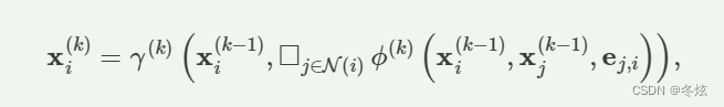
上面公式就是常见的节点更新公式。其中k 为图层的序号。r 为更新公式，就是邻居信息和之间边的信息的聚合表示。 正方形代表聚集邻居信息成一个向量。i 代表当前节点序号。j 为邻居节点序号。

2. 一些基础类

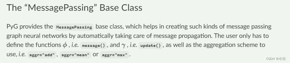 Message Passing 基础类就可以满足上面公式的实现，其中我们可以自定义 邻居及边融合的函数message() 和当前节点的更新公式update() 例如 add  mean  max

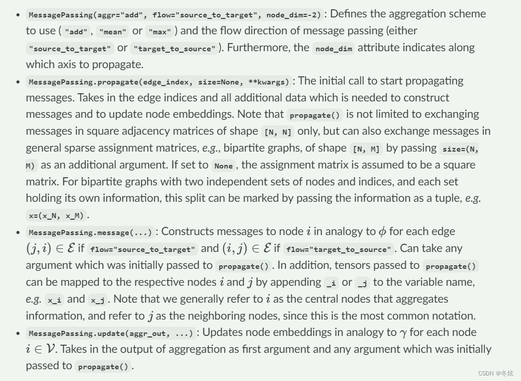
 MessagePassing(aggr = "add", flow="source_to_target", node_dim=2)

我认为应该指的就是上面的公式，node_dim 指的应该在哪个维度聚合。当然是节点个数的那个维度，最后一个维度是节点的特征维度所以最终选择 -2

然后介绍了一些message 和update函数的细节。感觉具体的参数传递还是得看例子中如何调用。

Let us verify this by re-implementing two popular GNN variants, the GCN layer from Kipf and Welling and the EdgeConv layer from Wang et al..

3. 实现一个GCN Layer层

 

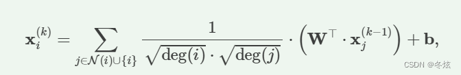
 上面就是需要实现的更新公式

我们可以看到邻居节点与本身节点序号合并，也就是有自环

1. Add self-loops to the adjacency matrix. 首先加入自环 边

2. Linearly transform node feature matrix. W 的矩阵实现，线性层

3. Compute normalization coefficients. 入度出度计算

4. Normalize node features in ϕ. 构成归一化项（分母）

5. Sum up neighboring node features ("add" aggregation). 将邻居节点及自己的特征相加

6. Apply a final bias vector.  应用一个 b  向量。

其中4，5 会涉及到上面的基础类MessagePassing. 1-3 只是特征预处理阶段 

import torch
from torch.nn import Linear, Parameter
from torch_geometric.nn import MessagePassing
from torch_geometric.utils import add_self_loops, degree

class GCNConv(MessagePassing):
    def __init__(self, in_channels, out_channels):
        super().__init__(aggr='add')  # "Add" aggregation (Step 5).
        self.lin = Linear(in_channels, out_channels, bias=False) # bias 只是最后加
        self.bias = Parameter(torch.Tensor(out_channels)) #这就是最后加入的bias， 维度就是输出的节点特征维度

        self.reset_parameters()#重置学习的参数和bias

    def reset_parameters(self):
        self.lin.reset_parameters()
        self.bias.data.zero_()

    def forward(self, x, edge_index):
        # x has shape [N, in_channels] 就是一个mini batch 的 大图。N 指的就是节点个数，in_channels 就是输入节点的特征维度
        # edge_index has shape [2, E] 就是边的稀疏连接矩阵

        # Step 1: Add self-loops to the adjacency matrix.
        edge_index, _ = add_self_loops(edge_index, num_nodes=x.size(0))# 直接利用函数，就可以在原先的节点边的链表中添加 自环边。操作应该就是 append 对应扩展。x.size(0)指的就是大图的节点个数

        # Step 2: Linearly transform node feature matrix.
        x = self.lin(x) 

        # Step 3: Compute normalization.
        row, col = edge_index #按照方向，应该是row 指的是源节点邻居节点，col 指的是当前节点，row 是箭头的始端，col 是箭头的尾端
        deg = degree(col, x.size(0), dtype=x.dtype)# 这样如果是有向图，应该就是入度
        deg_inv_sqrt = deg.pow(-0.5) 
        deg_inv_sqrt[deg_inv_sqrt == float('inf')] = 0 # 指的对有些节点没有边入的处理。1/0 的除不尽用0 表示，也就是归一化系数为0 。
        norm = deg_inv_sqrt[row] * deg_inv_sqrt[col] # 根据边  将每个边的归一化系数求出。

        # Step 4-5: Start propagating messages.
        out = self.propagate(edge_index, x=x, norm=norm)
# 这里我们要注意的就是propagate的参数维度。edge_index [2, E], x 还是[N, out_channels],norm 是[E, ]

        # Step 6: Apply a final bias vector.
        out += self.bias

        return out

    def message(self, x_j, norm):
        # x_j has shape [E, out_channels]

        # Step 4: Normalize node features.
        return norm.view(-1, 1) * x_j

We then call propagate(), which internally calls message(), aggregate() and update(). 

propagate 中间会自动调用 message 、aggregate 、 update 函数们。

外层调用咱门编写的GCN Conv类

conv = GCNConv(16, 32)
x = conv(x, edge_index)