sklearn SVM使用

SVM分类

线性SVM分类

• SVM是二分类器，线性SVM分类是画出一条决策边界，使得到两个类样本的最短距离最大。
• 主要有hard margin classification与soft margin classification，可以通过调节超参数来调节margin
• SVM直接输出样本的列别，而不是像Logistic回归那样，输出概率
• sklearn中，有多种方式实现线性SVM
  
  • LinearSVC
  • SVC中，kernel设置为linear
  • SGDClassifier中，loss设置为hinge，alpha设置为1/(m*C)

import numpy as np
from sklearn import datasets
from sklearn.pipeline import Pipeline
from sklearn.preprocessing import StandardScaler
from sklearn.svm import LinearSVC

iris = datasets.load_iris()
X = iris["data"][:, (2,3)]
y = (iris["target"] == 2).astype( np.float64 )

svm_clf = Pipeline(( ("scaler", StandardScaler()),
                     ("linear_svc", LinearSVC(C=1, loss="hinge")) ,))

svm_clf.fit( X, y )
res = svm_clf.predict( [[5.5, 1.7]] )

print( res )

[ 1.]

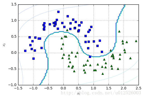
非线性SVM

• 一般现实问题中，线性模型难以解决问题，可以采用非线性SVM
• 对于非线性回归问题，可以先添加一个多项式的特征，即将一维数据转化为多项式数据，然后采用线性SVM；或者也可以直接采用多项式的kernel，直接进行非线性SVM的分类
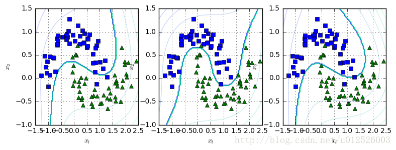
• SVC中的参数C越大，对于训练集来说，其误差越小，但是很容易发生过拟合；C越小，则允许有更多的训练集误分类，相当于soft margin
• SVC中的参数coef0反映了高阶多项式相对于低阶多项式对模型的影响，如果发生了过拟合的现象，则可以减小coef0；如果发生了欠拟合的现象，可以试着增大coef0

%matplotlib inline
import matplotlib.pyplot as plt
from sklearn.datasets import make_moons
from sklearn.preprocessing import PolynomialFeatures
X, y = make_moons( n_samples=100, noise=0.15, random_state=42 )

def plot_dataset(X, y, axes):
    plt.plot( X[:,0][y==0], X[:,1][y==0], "bs" )
    plt.plot( X[:,0][y==1], X[:,1][y==1], "g^" )
    plt.axis( axes )
    plt.grid( True, which="both" )
    plt.xlabel(r"$x_l$")
    plt.ylabel(r"$x_2$")

# contour函数是画出轮廓，需要给出X和Y的网格，以及对应的Z，它会画出Z的边界（相当于边缘检测及可视化）
def plot_predict(clf, axes):
    x0s = np.linspace(axes[0], axes[1], 100)
    x1s = np.linspace(axes[2], axes[3], 100)
    x0, x1 = np.meshgrid( x0s, x1s )
    X = np.c_[x0.ravel(), x1.ravel()]
    y_pred = clf.predict( X ).reshape( x0.shape )
    y_decision = clf.decision_function( X ).reshape( x0.shape )
    plt.contour( x0, x1, y_pred, cmap=plt.cm.winter, alpha=0.5 )
    plt.contour( x0, x1, y_decision, cmap=plt.cm.winter, alpha=0.2 )

polynomial_svm_clf = Pipeline([ ("poly_featutres", PolynomialFeatures(degree=3)),
                                ("scaler", StandardScaler()),
                                ("svm_clf", LinearSVC(C=10, loss="hinge", random_state=42)  )
                            ])
polynomial_svm_clf.fit( X, y )
plot_dataset( X, y, [-1.5, 2.5, -1, 1.5] )
plot_predict( polynomial_svm_clf, [-1.5, 2.5, -1, 1.5] )
plt.show()

from sklearn.svm import SVC
poly_kernel_svm_clf = Pipeline([ ( "scaler", StandardScaler()),
                                 ("svm_clf", SVC(kernel="poly", degree=3, coef0=1, C=0.5))
                                ])
poly_kernel_svm_clf.fit(X,y)
plt.figure( figsize=(9,3) )
plt.subplot(131)
plot_dataset( X, y, [-1.5, 2.5, -1, 1.5] )
plot_predict( poly_kernel_svm_clf, [-1.5, 2.5, -1, 1.5] )
# plt.show()

poly_kernel_svm_clf = Pipeline([ ( "scaler", StandardScaler()),
                                 ("svm_clf", SVC(kernel="poly", degree=3, coef0=1, C=10))
                                ])
poly_kernel_svm_clf.fit(X,y)
plt.subplot(132)
plot_dataset( X, y, [-1.5, 2.5, -1, 1.5] )
plot_predict( poly_kernel_svm_clf, [-1.5, 2.5, -1, 1.5] )

poly_kernel_svm_clf = Pipeline([ ( "scaler", StandardScaler()),
                                 ("svm_clf", SVC(kernel="poly", degree=3, coef0=100, C=0.5))
                                ])
poly_kernel_svm_clf.fit(X,y)
plt.subplot(133)
plot_dataset( X, y, [-1.5, 2.5, -1, 1.5] )
plot_predict( poly_kernel_svm_clf, [-1.5, 2.5, -1, 1.5] )

plt.show()

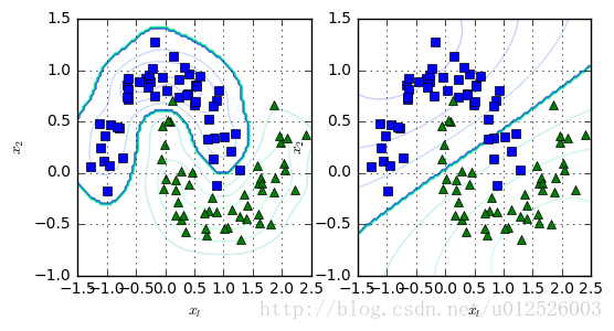
Gasuusian RBF核函数

• 当数据在低维空间中不可分割的时候，可以尝试将它们映射到高维空间，通过核函数来进行这样的映射操作，Gaussian RBF核函数为
  $$\phi \gamma (x,l) = {e^{( - \gamma {{\left\| {x - l} \right\|}^2})}}$$

复杂度分析

• skleanr中，SVM是利用了libsvm，线性SVM的时间复杂度为$O(mn)$，带有核函数的SVM一般是$O(m^2 n)$与$O(m^3 n)$之间
• SVM一般适用于数据量不是很大，但是很复杂的问题的求解。

rbf_kernel_svm_clf = Pipeline([
                                ("scaler", StandardScaler()), 
                                ("svm_clf", SVC(kernel="rbf", gamma=5, C=0.001))
                            ])

plt.figure(figsize=(6,3))
plt.subplot(121)
rbf_kernel_svm_clf.fit( X, y )
plot_dataset( X, y, [-1.5, 2.5, -1, 1.5] )
plot_predict( rbf_kernel_svm_clf, [-1.5, 2.5, -1, 1.5] )

rbf_kernel_svm_clf = Pipeline([
                                ("scaler", StandardScaler()), 
                                ("svm_clf", SVC(kernel="rbf", gamma=0.1, C=0.001))
                            ])
plt.subplot(122)
rbf_kernel_svm_clf.fit( X, y )
plot_dataset( X, y, [-1.5, 2.5, -1, 1.5] )
plot_predict( rbf_kernel_svm_clf, [-1.5, 2.5, -1, 1.5] )
plt.show(  )

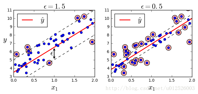
SVM回归

线性SVM

• SVM也可以用于回归问题，有线性SVM与非线性SVM回归
• 线性回归时，有一个变量$\varepsilon$，这是SVM的margin

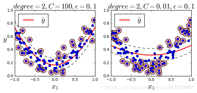
非线性SVM回归

• 多项式回归，指定SVM的kernel为poly即可

from sklearn.svm import LinearSVR
np.random.seed( 42 )
m = 50
X = 2*np.random.rand(m, 1)
y = (4+3*X+np.random.randn(m,1)).ravel()

# 找到训练集中所有支持向量的下标
def find_support_vectors(svm_reg, X, y):
    y_pred = svm_reg.predict( X )
    off_margin = np.abs(y-y_pred) >= svm_reg.epsilon
    # 返回off_margin中值为True的下标
    return np.argwhere( off_margin )

def plot_svm_regression( svm_reg, X, y, axes ):
    x1s = np.linspace( axes[0], axes[1], 100 ).reshape(-1,1)
    y_pred = svm_reg.predict(x1s)
    plt.plot( x1s, y_pred, "r-", linewidth=2, label=r"$\hat{y}$" )
    plt.plot( x1s, y_pred-svm_reg.epsilon, "k--" )
    plt.plot( x1s, y_pred+svm_reg.epsilon, "k--" )
    plt.plot( X, y, "bo" )
    plt.scatter( X[svm_reg.support_], y[svm_reg.support_], s=180, facecolors="#FFAAAA" )
    plt.xlabel(r"$x_1$", fontsize=18)
    plt.legend(loc="upper left", fontsize=18)
    plt.axis(axes)


svm_reg_1 = LinearSVR(epsilon=1.5, random_state=42)
svm_reg_2 = LinearSVR(epsilon=0.5, random_state=42)
svm_reg_1.fit( X, y )
svm_reg_2.fit( X, y )

svm_reg_1.support_ = find_support_vectors( svm_reg_1, X, y )
svm_reg_2.support_ = find_support_vectors( svm_reg_2, X, y )

eps_x1 = 1
eps_y_pred = svm_reg_1.predict([[eps_x1]])

plt.figure( figsize=(8,3) )
plt.subplot(121)
plot_svm_regression( svm_reg_1, X, y, [0, 2, 3, 11] )
plt.title(r"$\epsilon = {}$".format(svm_reg_1.epsilon), fontsize=18)
plt.ylabel(r"$y$", fontsize=18, rotation=0)
plt.annotate(
        '', xy=(eps_x1, eps_y_pred), xycoords='data',
        xytext=(eps_x1, eps_y_pred - svm_reg_1.epsilon),
        textcoords='data', arrowprops={'arrowstyle': '<->', 'linewidth': 1.5}
    )
plt.text(0.9, 5.6, r"$\epsilon$", fontsize=20)

plt.subplot(122)
plot_svm_regression(svm_reg_2, X, y, [0, 2, 3, 11])
plt.title(r"$\epsilon = {}$".format(svm_reg_2.epsilon), fontsize=18)
plt.show()

from sklearn.svm import SVR

np.random.seed(42)
m = 100
X = 2 * np.random.rand(m, 1) - 1
y = (0.2 + 0.1 * X + 0.5 * X**2 + np.random.randn(m, 1)/10).ravel()

svm_poly_reg1 = SVR(kernel="poly", degree=2, C=100, epsilon=0.1)
svm_poly_reg2 = SVR(kernel="poly", degree=2, C=0.01, epsilon=0.1)
svm_poly_reg1.fit(X, y)
svm_poly_reg2.fit(X, y)

plt.figure(figsize=(8, 3))
plt.subplot(121)
plot_svm_regression(svm_poly_reg1, X, y, [-1, 1, 0, 1])
plt.title(r"$degree={}, C={}, \epsilon = {}$".format(svm_poly_reg1.degree, svm_poly_reg1.C, svm_poly_reg1.epsilon), fontsize=18)
plt.ylabel(r"$y$", fontsize=18, rotation=0)
plt.subplot(122)
plot_svm_regression(svm_poly_reg2, X, y, [-1, 1, 0, 1])
plt.title(r"$degree={}, C={}, \epsilon = {}$".format(svm_poly_reg2.degree, svm_poly_reg2.C, svm_poly_reg2.epsilon), fontsize=18)
plt.show()

SVM的一些探讨

• hard margin模式时，线性SVM分类的预测方法为
  $$\hat y = \left\{ \begin{array}{l} 0 & if{\kern 1pt} {w^T}x + b < 0,\\ 1 & if{\kern 1pt} {w^T}x + b \ge 0 \end{array} \right.$$
• 减小权重，会增大margin
• software margin的SVM分类器的目标函数为
  $$\begin{array}{l} \mathop {\min }\limits_{w,b,\zeta } & \frac{1}{2}{w^T}w + C\sum\limits_{i = 1}^m {{\zeta ^{(i)}}} \\ s.t. & {t^{(i)}}({w^T}{x^{(i)}} + b) \ge 1 - {\zeta ^{(i)}} & and & {\zeta ^{(i)}} \ge 0{\kern 1pt} for{\kern 1pt} {\kern 1pt} i = 1,2, \cdots ,m \end{array}$$
  可以将原始问题转化为对偶问题
• 对于kernel SVM来说，解决方法也是类似，不过可以化简核函数对样本之间的求解
• SVM一般是offline的，因为训练SVM可以需要大量时间，如果需要online SVM，即模型随着数据量的不断增加而不断改进，有一种原始的方法是使用梯度下降的方法，最小化代价函数，但是这种方法的收敛速度远小于QP方法
• 关于SVM更多的推导：http://www.cnblogs.com/LeftNotEasy/archive/2011/05/02/basic-of-svm.html