ARIMA模型

ARIMA模型

简介

• ARIMA模型是由AR、I与MA模型组成
• AR(p)：auto regressive，自回归模型，表示当前的数值与过去p个时间节点的值的回归，不依赖别的值，所以称为自回归；其中$p$称为自回归的阶数。
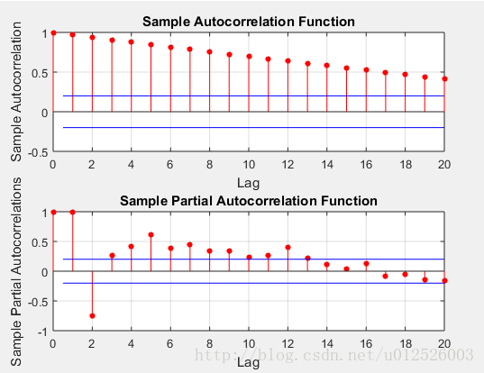
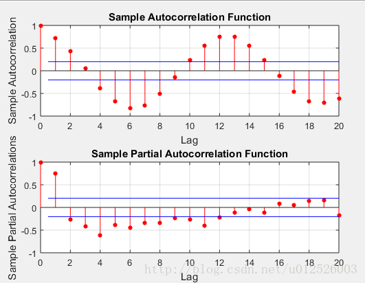
• I(d)：integrateed，有的时间序列不是平稳信号，使用对数或者差分的方法可是将数据转化为平稳数据，数据的平稳性可以用数据的ACF(自相关)与PACF(偏自相关)图去判断。$d$是差分的阶数
• MA(q)：moving average，移动平均模型，表示当前的值，是过去q个时间点的预测误差的回归。 q q <script type="math/tex" id="MathJax-Element-189">q</script>是MA的移动平均的阶数
• 具体的公式参考链接：http://danzhuibing.github.io/ml_arima_basic.html
• 关于ACF与PACF的解释：http://www.cnblogs.com/tongji-wu/p/3439372.html

代码

%%
clc,clear,close all

t = 1:100;
t = t';
y = 2*t + 10*sin(t/2) + randn( size(t) );
figure
plot( t, y )

%% ACF和PACF 
figure
subplot(211),autocorr( y );
subplot(212),parcorr( y );
figure
dy = diff( y );
subplot(211),autocorr( dy );
subplot(212),parcorr( dy );

%% ARIMA 模型
Mdl = arima(5,1,0);
EstMdl = estimate(Mdl,y);
res = infer(EstMdl,y);
% 模型验证
figure
subplot(2,2,1)
plot(res./sqrt(EstMdl.Variance))
title('Standardized Residuals')
subplot(2,2,2),qqplot(res)
subplot(2,2,3),autocorr(res)
subplot(2,2,4),parcorr(res)
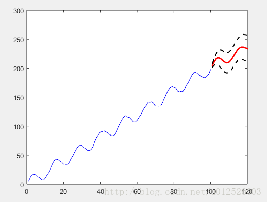
% 预测
[yF,yMSE] = forecast(EstMdl,20,'Y0',y);
UB = yF + 1.96*sqrt(yMSE);
LB = yF - 1.96*sqrt(yMSE);

figure
h4 = plot(y,'b');
hold on
h5 = plot(101:120,yF,'r','LineWidth',2);
h6 = plot(101:120,UB,'k--','LineWidth',1.5);
plot(101:120,LB,'k--','LineWidth',1.5);
hold off

• 首先观察数据是否为平稳序列，如果不是，则需要使用差分等方法进行转化，才能使用ARMA模型
• 一些结果

• 原始图像
  

• 原始数据的ACF与PACF
  

• 原始数据差分后的ACF与PACF
  
• 模型验证
  
• 模型预测