深度学习目标检测Yolo算法代码实现

最新推荐文章于 2024-05-09 16:10:48 发布

RyanC3

最新推荐文章于 2024-05-09 16:10:48 发布

阅读量6.3k

点赞数 8

文章标签：深度学习算法目标检测

本文链接：https://blog.csdn.net/u012655441/article/details/121141084

版权

前言

本篇博客主要是根据yolo系列的算法代码，总结Yolo系列用到的技术，包括anchor box设置，数据的读入以及处理，即插即用的注意力机制模块、loss function设置等。本篇博客主要根据的代码来源是Yolov3和Yolov4，代码都是基于tensorflow框架的，原理可以参考我之前写的一些博客：目标检测综述、目标检测yolo系列和目标检测YOLO系列算法。相关的论文：Yolov3和Yolov4。原版的代码：Yolov4和Yolov3.Yolov4详细请参考我的git仓库的Readme.md文件。

Yolov3

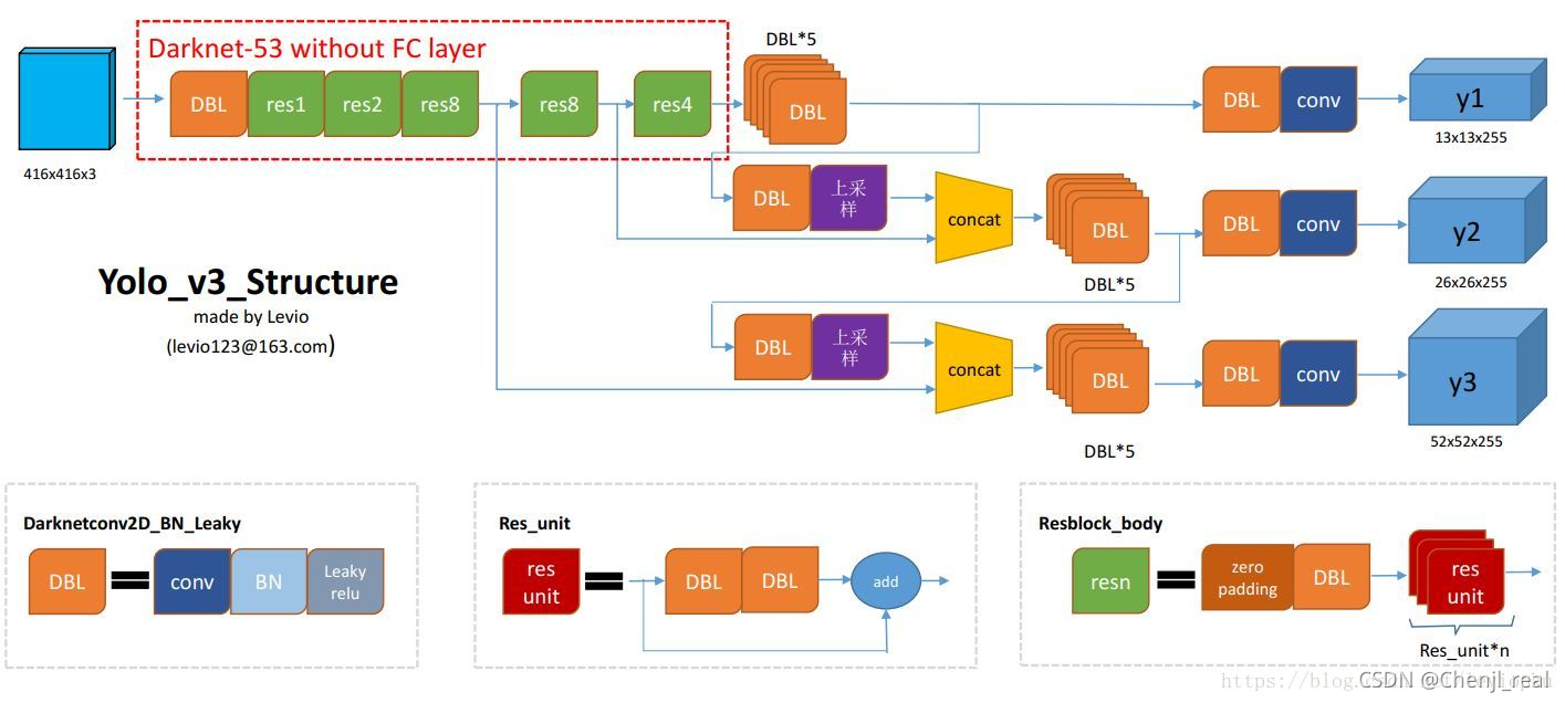
Yolov3的网络结构图如下图所示：
在这里插入图片描述

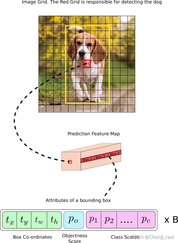
Anchor设置

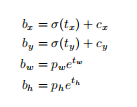
$C_x$ 和 $C_y$ 表示待检测目标中心点的坐标所在的grid的左上角的坐标，下图 $C_x$ 和 $C_y$ 则为（1，1）。 $\sigma(t_x)$ 和 $\sigma(t_y)$ 表示偏移量，用sigmoid将tx,ty压缩到[0,1]区间內，可以有效的确保目标中心处于执行预测的网格单元中，防止偏移过多。 $P_w$ 和 $P_h$ 表示anchor box映射到feature map中的宽和高，用到指数是因为 $t_w$ , $t_h$ 是 $\log$ 尺度缩放到对数空间。终得到的边框坐标值是 $b_x$ , $b_y$ , $b_w$ , $b_h$ 即边界框bbox相对于feature map的位置和大小，是模型需要的预测输出坐标。但网络实际上的学习目标是 $t_x$ , $t_y$ , $t_w$ , $t_h$ 这４个offsets，其中 $t_x$ , $t_y$ 是预测的坐标偏移值， $t_w$ , $t_h$ 是尺度缩放，有了这４个offsets，自然可以根据之前的公式去求得真正需要的 $b_x$ , $b_y$ , $b_w$ , $b_h$ ４个坐标。关于图像的缩放同时需要保持图像的长宽比例，然后用padding进行补充。
在这里插入图片描述

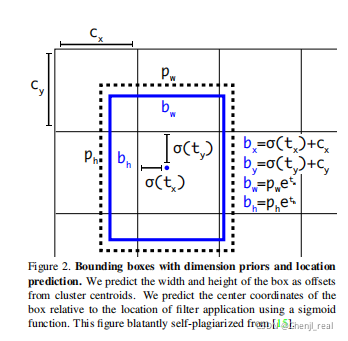
在yolov3中与faster-rcnn系列文章用到的公式在前两行是不同的，yolov3里 $P_x$ 和 $P_y$ 就换为了feature map上的grid cell左上角坐标 $C_x$ , $C_y$ 了，即在yolov3里是 $G_x$ , $G_y$ 减去grid cell左上角坐标 $C_x$ , $C_y$ 。 $x$ , $y$ 坐标并没有针对anchon box求偏移量，所以并不需要除以 $P_w$ , $P_h$ 。也就是 $t_x = G_x - C_x$ ， $t_y = G_y - C_y$ 这样就可以直接求bbox中心距离grid cell左上角的坐标的偏移量。 $t_w$ 和 $t_h$ 的公式yolov3和faster-rcnn系列是一样的，是物体所在边框的长宽和anchor box长宽之间的比率，不管Faster-RCNN还是YOLO，都不是直接回bounding box的长宽而是尺度缩放到对数空间，是怕训练会带来不稳定的梯度。因为如果不做变换，直接预测相对形变 $t_w$ ，那么要求 $t_w>0$ ，因为框的宽高不可能是负数。这样，是在做一个有不等式条件约束的优化问题，没法直接用SGD来做。所以先取一个对数变换，将其不等式约束去掉。

在这里插入图片描述

Anchor box的作用是第一是提高召回率，当多个目标中心位于同一个cell内时，不同比例的预测框可以预测不同类别的物体。第二是降低学习难度，anchor给出目标宽高的绝对量，只需要回归偏移量即可。

在这里插入图片描述

Anchor计算

设矩形框的面积为 $s$ ，矩形框的宽为 $w$ ，高为 $h$ ，则有： $\{^{w\times h = s}_{\frac{w}{h}=ratio} \Rightarrow \{^{w = ratio \cdot h}_{ratio\times h^2 = s}$ 最终得到： $\{^{h = \sqrt{s/ratio}}_{w=ratio\cdot h = \sqrt{s\cdot ratio}}$ 不同尺度上缩放scale，则有： $\{^{h = \sqrt{sacle\cdot s/ratio}}_{w=ratio\cdot h = \sqrt{scale \cdot s\cdot ratio}}$

通过聚类生成anchor box

原理可以参考：K-means聚类生成Anchor box
要注意的是标准的K-means算法一般使用的是欧式距离作为样本的度量，在生成anchor box的任务中，并不能使用欧式距离，因为大小不一的anchor box的产生误差不一样，大box簇会比小box簇产生更大的误差。
代码如下：

#coding=utf-8
import xml.etree.ElementTree as ET
import numpy as np
import glob
import sys
sys.path.append('.')
import config as sys_config
from tqdm import tqdm
 
def iou(box, clusters):
    """
    计算一个ground truth边界盒和k个先验框(Anchor)的交并比(IOU)值。
    参数box: 元组或者数据，代表ground truth的长宽。
    参数clusters: 形如(k,2)的numpy数组，其中k是聚类Anchor框的个数
    返回：ground truth和每个Anchor框的交并比。
    """
    x = np.minimum(clusters[:, 0], box[0])
    y = np.minimum(clusters[:, 1], box[1])
    if np.count_nonzero(x == 0) > 0 or np.count_nonzero(y == 0) > 0:
        raise ValueError("Box has no area")
    interp = x * y
    box_area = box[0] * box[1]
    cluster_area = clusters[:, 0] * clusters[:, 1]
    iou_ = interp / (box_area + cluster_area - interp)
    return iou_
 
 
def avg_iou(boxes, clusters):
    """
    计算一个ground truth和k个Anchor的交并比的均值。
    """
    return np.mean([np.max(iou(boxes[i], clusters)) for i in range(boxes.shape[0])])
 
def kmeans(boxes, k, dist=np.median):
    """
    利用IOU值进行K-means聚类
    参数boxes: 形状为(r, 2)的ground truth框，其中r是ground truth的个数
    参数k: Anchor的个数
    参数dist: 距离函数
    返回值：形状为(k, 2)的k个Anchor框
    """
    # 即是上面提到的r
    rows = boxes.shape[0]
    # 距离数组，计算每个ground truth和k个Anchor的距离
    distances = np.empty((rows, k))
    # 上一次每个ground truth"距离"最近的Anchor索引
    last_clusters = np.zeros((rows,))
    # 设置随机数种子
    np.random.seed()
 
    # 初始化聚类中心，k个簇，从r个ground truth随机选k个
    clusters = boxes[np.random.choice(rows, k, replace=False)]
    # 开始聚类
    while True:
        # 计算每个ground truth和k个Anchor的距离，用1-IOU(box,anchor)来计算
        for row in range(rows):
            distances[row] = 1 - iou(boxes[row], clusters)
        # 对每个ground truth，选取距离最小的那个Anchor，并存下索引
        nearest_clusters = np.argmin(distances, axis=1)
        # 如果当前每个ground truth"距离"最近的Anchor索引和上一次一样，聚类结束
        if (last_clusters == nearest_clusters).all():
            break
        # 更新簇中心为簇里面所有的ground truth框的均值
        for cluster in range(k):
            clusters[cluster] = dist(boxes[nearest_clusters == cluster], axis=0)
        # 更新每个ground truth"距离"最近的Anchor索引
        last_clusters = nearest_clusters
 
    return clusters
 
# 加载自己的数据集，只需要所有labelimg标注出来的xml文件即可
def load_dataset(path):
    dataset = []
    for xml_file in tqdm(glob.glob("{}/*xml".format(path))):
        tree = ET.parse(xml_file)
        # 图片高度
        height = int(tree.findtext("./size/height"))
        # 图片宽度
        width = int(tree.findtext("./size/width"))
        
        for obj in tree.iter("object"):
            # 偏移量
            xmin = int(obj.findtext("bndbox/xmin")) / width
            ymin = int(obj.findtext("bndbox/ymin")) / height
            xmax = int(obj.findtext("bndbox/xmax")) / width
            ymax = int(obj.findtext("bndbox/ymax")) / height
            xmin = np.float64(xmin)
            ymin = np.float64(ymin)
            xmax = np.float64(xmax)
            ymax = np.float64(ymax)
            if xmax == xmin or ymax == ymin:
                print(xml_file)
            # 将Anchor的长宽放入dateset，运行kmeans获得Anchor
            dataset.append([xmax - xmin, ymax - ymin])
    return np.array(dataset)
 
if __name__ == '__main__':
    import os
    ANNOTATIONS_PATH = os.path.join(sys_config.dataset_base_path, 'Annotations')
    # ANNOTATIONS_PATH = r'D:\Datasets\VOC\VOCtest_06-Nov-2007\VOCdevkit\VOC2007\Annotations'
    CLUSTERS = 9 #聚类数量，anchor数量
    INPUTDIM = sys_config.imagesize #输入网络大小
 
    data = load_dataset(ANNOTATIONS_PATH)
    out = kmeans(data, k=CLUSTERS)
    print('Boxes:')
    print(np.array(out)*INPUTDIM)
    print("Accuracy: {:.2f}%".format(avg_iou(data, out) * 100))       
    final_anchors = np.around(out[:, 0] / out[:, 1], decimals=2).tolist()
    print("Before Sort Ratios:\n {}".format(final_anchors))
    print("After Sort Ratios:\n {}".format(sorted(final_anchors)))

数据处理

转换成tfrecord格式数据

在代码Yolov3里面，数据的格式是采样tfrecord进行输入。TFRecord是Google官方推荐的一种数据格式，实际上它是一种二进制文件，其能更好地利用内存，其内部包含了多个tf.train.Example，而Example是protocol buffer数据标准的实现，在一个Example消息体重包含了一系列的tf.train.feature属性，每一个feature是一个key-value形式的键值对。value的取值有以下三种：

bytes_list：可以存储string和byte两种数据类型。
float_list：可以存储float(float32)与double(float64)两种数据类型。
int64_list：可以存储bool，enum，int32，uint32，int64，uint64

生成tfrecord的代码：

#该函数传入的是xml里面的annotation，class_map表示classid：以及class_name
def build_example(annotation, class_map):
    img_path = os.path.join(
        FLAGS.data_dir, 'JPEGImages', annotation['filename'])
    print(img_path)
    img_raw = open(img_path, 'rb').read()
    key = hashlib.sha256(img_raw).hexdigest()

    width = int(annotation['size']['width'])
    height = int(annotation['size']['height'])

    xmin = []
    ymin = []
    xmax = []
    ymax = []
    classes = []
    classes_text = []
    truncated = []
    views = []
    difficult_obj = []
    if 'object' in annotation:
        for obj in annotation['object']:
            difficult = bool(int(obj['difficult']))
            difficult_obj.append(int(difficult))

            xmin.append(float(obj['bndbox']['xmin']) / width)
            ymin.append(float(obj['bndbox']['ymin']) / height)
            xmax.append(float(obj['bndbox']['xmax']) / width)
            ymax.append(float(obj['bndbox']['ymax']) / height)
            classes_text.append(obj['name'].encode('utf8'))
            classes.append(class_map[obj['name']])
            truncated.append(int(obj['truncated']))
            views.append(obj['pose'].encode('utf8'))

    example = tf.train.Example(features=tf.train.Features(feature={
        'image/height': tf.train.Feature(int64_list=tf.train.Int64List(value=[height])),
        'image/width': tf.train.Feature(int64_list=tf.train.Int64List(value=[width])),
        'image/filename': tf.train.Feature(bytes_list=tf.train.BytesList(value=[
            annotation['filename'].encode('utf8')])),
        'image/source_id': tf.train.Feature(bytes_list=tf.train.BytesList(value=[
            annotation['filename'].encode('utf8')])),
        'image/key/sha256': tf.train.Feature(bytes_list=tf.train.BytesList(value=[key.encode('utf8')])),
        'image/encoded': tf.train.Feature(bytes_list=tf.train.BytesList(value=[img_raw])),
        'image/format': tf.train.Feature(bytes_list=tf.train.BytesList(value=['jpeg'.encode('utf8')])),
        'image/object/bbox/xmin': tf.train.Feature(float_list=tf.train.FloatList(value=xmin)),
        'image/object/bbox/xmax': tf.train.Feature(float_list=tf.train.FloatList(value=xmax)),
        'image/object/bbox/ymin': tf.train.Feature(float_list=tf.train.FloatList(value=ymin)),
        'image/object/bbox/ymax': tf.train.Feature(float_list=tf.train.FloatList(value=ymax)),
        'image/object/class/text': tf.train.Feature(bytes_list=tf.train.BytesList(value=classes_text)),
        'image/object/class/label': tf.train.Feature(int64_list=tf.train.Int64List(value=classes)),
        'image/object/difficult': tf.train.Feature(int64_list=tf.train.Int64List(value=difficult_obj)),
        'image/object/truncated': tf.train.Feature(int64_list=tf.train.Int64List(value=truncated)),
        'image/object/view': tf.train.Feature(bytes_list=tf.train.BytesList(value=views)),
    }))
    return example

通过以下函数可以查看tfrecord到底记录了什么：

# 解析parse_tfrecord
def parse_tfrecord(tfrecord, class_table, size):
    x = tf.io.parse_single_example(tfrecord, IMAGE_FEATURE_MAP)
    x_train = tf.image.decode_jpeg(x['image/encoded'], channels=3)
    x_train = tf.image.resize(x_train, (size, size))

    class_text = tf.sparse.to_dense(
        x['image/object/class/text'], default_value='')
    labels = tf.cast(class_table.lookup(class_text), tf.float32)
    y_train = tf.stack([tf.sparse.to_dense(x['image/object/bbox/xmin']),
                        tf.sparse.to_dense(x['image/object/bbox/ymin']),
                        tf.sparse.to_dense(x['image/object/bbox/xmax']),
                        tf.sparse.to_dense(x['image/object/bbox/ymax']),
                        labels], axis=1)

    paddings = [[0, FLAGS.yolo_max_boxes - tf.shape(y_train)[0]], [0, 0]]
    y_train = tf.pad(y_train, paddings)

    return x_train, y_train
def load_tfrecord_dataset(file_pattern, class_file, size=416):
    LINE_NUMBER = -1  # TODO: use tf.lookup.TextFileIndex.LINE_NUMBER
    '''
    tf.lookup.StaticHashTable：建立类别与数字的关联关系
    keys_tensor = tf.constant([1, 2])
    vals_tensor = tf.constant([3, 4])
    input_tensor = tf.constant([1, 5])
    table = tf.lookup.StaticHashTable(
    tf.lookup.KeyValueTensorInitializer(keys_tensor, vals_tensor), -1)
    print(table.lookup(input_tensor))
    output:tf.Tensor([ 3 -1], shape=(2,), dtype=int32)

    tf.lookup.TextFileInitializer：Table initializers from a text file.
    '''
    class_table = tf.lookup.StaticHashTable(tf.lookup.TextFileInitializer(
        class_file, tf.string, 0, tf.int64, LINE_NUMBER, delimiter="\n"), -1)

    files = tf.data.Dataset.list_files(file_pattern)
    dataset = files.flat_map(tf.data.TFRecordDataset)
    return dataset.map(lambda x: parse_tfrecord(x, class_table, size))

import sys
import os
path = os.path.abspath(os.path.join(os.getcwd()))
sys.path.append(path)
print(sys.path)
import time
from absl import app, flags, logging
from absl.flags import FLAGS
import cv2
import numpy as np
import tensorflow as tf
from yolov3_tf2.models import (
    YoloV3, YoloV3Tiny
)
from yolov3_tf2.dataset import load_tfrecord_dataset, transform_images
from yolov3_tf2.utils import draw_outputs

flags.DEFINE_string('classes', './data/voc2012_trainbin.names', 'path to classes file')
flags.DEFINE_integer('size', 416, 'resize images to')
flags.DEFINE_string(
    'dataset', './data/voc_train_trashBin.tfrecord', 'path to dataset')
flags.DEFINE_string('output', './output.jpg', 'path to output image')


def main(_argv):
    class_names = [c.strip() for c in open(FLAGS.classes).readlines()]
    logging.info('classes loaded')
    dataset = load_tfrecord_dataset(FLAGS.dataset, FLAGS.classes, FLAGS.size)
    dataset = dataset.shuffle(512)
    for image, labels in dataset.take(4):
        boxes = []
        scores = []
        classes = []
        for x1, y1, x2, y2, label in labels:
            if x1 == 0 and x2 == 0:
                continue

            boxes.append((x1, y1, x2, y2))
            scores.append(1)
            classes.append(label)
        nums = [len(boxes)]
        boxes = [boxes]
        scores = [scores]
        classes = [classes]

        logging.info('labels:')
        for i in range(nums[0]):
            logging.info('\t{}, {}, {}'.format(class_names[int(classes[0][i])],
                                               np.array(scores[0][i]),
                                               np.array(boxes[0][i])))

        img = cv2.cvtColor(image.numpy(), cv2.COLOR_RGB2BGR)
        img = draw_outputs(img, (boxes, scores, classes, nums), class_names)
        cv2.imwrite(FLAGS.output, img)
        logging.info('output saved to: {}'.format(FLAGS.output))


if __name__ == '__main__':
    app.run(main)

在这一块代码我还得要仔细看看。

加载数据

加载数据后需要进行分批，打乱，resize。

train_dataset = train_dataset.shuffle(buffer_size=512)
    train_dataset = train_dataset.batch(FLAGS.batch_size)
    train_dataset = train_dataset.map(lambda x, y: (
        dataset.transform_images(x, FLAGS.size),
        dataset.transform_targets(y, anchors, anchor_masks, FLAGS.size)))
    train_dataset = train_dataset.prefetch(
        buffer_size=tf.data.experimental.AUTOTUNE)

模型加载

Yolov3

其实对着上面的图看代码就非常容易理解。

def DarknetResidual(x, filters):
    prev = x
    x = DarknetConv(x, filters // 2, 1)
    x = DarknetConv(x, filters, 3)
    x = Add()([prev, x])
    return x


def DarknetBlock(x, filters, blocks):
    x = DarknetConv(x, filters, 3, strides=2)
    for _ in range(blocks):
        x = DarknetResidual(x, filters)
    return x


def Darknet(name=None):
    x = inputs = Input([None, None, 3])
    x = DarknetConv(x, 32, 3)
    x = DarknetBlock(x, 64, 1)
    x = DarknetBlock(x, 128, 2)  # skip connection
    x = x_36 = DarknetBlock(x, 256, 8)  # skip connection
    x = x_61 = DarknetBlock(x, 512, 8)
    x = DarknetBlock(x, 1024, 4)
    return tf.keras.Model(inputs, (x_36, x_61, x), name=name)

def YoloV3(size=None, channels=3, anchors=yolo_anchors,
           masks=yolo_anchor_masks, classes=80, training=False):
    x = inputs = Input([size, size, channels], name='input')

    x_36, x_61, x = Darknet(name='yolo_darknet')(x)

    x = YoloConv(512, name='yolo_conv_0')(x)
    output_0 = YoloOutput(512, len(masks[0]), classes, name='yolo_output_0')(x)
	# 这里做了concat
    x = YoloConv(256, name='yolo_conv_1')((x, x_61))
    output_1 = YoloOutput(256, len(masks[1]), classes, name='yolo_output_1')(x)
	# 这里做了concat，用到python里面的函数定义函数。
    x = YoloConv(128, name='yolo_conv_2')((x, x_36))
    output_2 = YoloOutput(128, len(masks[2]), classes, name='yolo_output_2')(x)
	# 如果需要训练的话则返回模型，否则返回输出
    if training:
        return Model(inputs, (output_0, output_1, output_2), name='yolov3')

    boxes_0 = Lambda(lambda x: yolo_boxes(x, anchors[masks[0]], classes),
                     name='yolo_boxes_0')(output_0)
    boxes_1 = Lambda(lambda x: yolo_boxes(x, anchors[masks[1]], classes),
                     name='yolo_boxes_1')(output_1)
    boxes_2 = Lambda(lambda x: yolo_boxes(x, anchors[masks[2]], classes),
                     name='yolo_boxes_2')(output_2)

    outputs = Lambda(lambda x: yolo_nms(x, anchors, masks, classes),
                     name='yolo_nms')((boxes_0[:3], boxes_1[:3], boxes_2[:3]))

    return Model(inputs, outputs, name='yolov3')

# As tensorflow lite doesn't support tf.size used in tf.meshgrid, 
# we reimplemented a simple meshgrid function that use basic tf function.
def _meshgrid(n_a, n_b):

    return [
        tf.reshape(tf.tile(tf.range(n_a), [n_b]), (n_b, n_a)),
        tf.reshape(tf.repeat(tf.range(n_b), n_a), (n_b, n_a))
    ]


def yolo_boxes(pred, anchors, classes):
    # pred: (batch_size, grid, grid, anchors, (x, y, w, h, obj, ...classes))
    grid_size = tf.shape(pred)[1:3]
    box_xy, box_wh, objectness, class_probs = tf.split(
        pred, (2, 2, 1, classes), axis=-1)
    # 将预测的数据归一化到[0, 1]区间
    box_xy = tf.sigmoid(box_xy)
    objectness = tf.sigmoid(objectness)
    class_probs = tf.sigmoid(class_probs)
    pred_box = tf.concat((box_xy, box_wh), axis=-1)  # original xywh for loss

    # !!! grid[x][y] == (y, x)
    grid = _meshgrid(grid_size[1],grid_size[0])
    grid = tf.expand_dims(tf.stack(grid, axis=-1), axis=2)  # [gx, gy, 1, 2]

    box_xy = (box_xy + tf.cast(grid, tf.float32)) / \
        tf.cast(grid_size, tf.float32)
    # 这个是因为在设置的时候已经被log了
    box_wh = tf.exp(box_wh) * anchors

    box_x1y1 = box_xy - box_wh / 2
    box_x2y2 = box_xy + box_wh / 2
    bbox = tf.concat([box_x1y1, box_x2y2], axis=-1)

    return bbox, objectness, class_probs, pred_box

训练

eager模式下即调试模式下写的代码，我怕是写不出这样的代码

    if FLAGS.mode == 'eager_tf':
        # Eager mode is great for debugging
        # Non eager graph mode is recommended for real training
        avg_loss = tf.keras.metrics.Mean('loss', dtype=tf.float32)
        avg_val_loss = tf.keras.metrics.Mean('val_loss', dtype=tf.float32)

        for epoch in range(1, FLAGS.epochs + 1):
            for batch, (images, labels) in enumerate(train_dataset):
                with tf.GradientTape() as tape:
                    outputs = model(images, training=True)
                    regularization_loss = tf.reduce_sum(model.losses)
                    pred_loss = []
                    for output, label, loss_fn in zip(outputs, labels, loss):
                        pred_loss.append(loss_fn(label, output))
                    total_loss = tf.reduce_sum(pred_loss) + regularization_loss

                grads = tape.gradient(total_loss, model.trainable_variables)
                optimizer.apply_gradients(
                    zip(grads, model.trainable_variables))

                logging.info("{}_train_{}, {}, {}".format(
                    epoch, batch, total_loss.numpy(),
                    list(map(lambda x: np.sum(x.numpy()), pred_loss))))
                avg_loss.update_state(total_loss)

            for batch, (images, labels) in enumerate(val_dataset):
                outputs = model(images)
                regularization_loss = tf.reduce_sum(model.losses)
                pred_loss = []
                for output, label, loss_fn in zip(outputs, labels, loss):
                    pred_loss.append(loss_fn(label, output))
                total_loss = tf.reduce_sum(pred_loss) + regularization_loss

                logging.info("{}_val_{}, {}, {}".format(
                    epoch, batch, total_loss.numpy(),
                    list(map(lambda x: np.sum(x.numpy()), pred_loss))))
                avg_val_loss.update_state(total_loss)

            logging.info("{}, train: {}, val: {}".format(
                epoch,
                avg_loss.result().numpy(),
                avg_val_loss.result().numpy()))

            avg_loss.reset_states()
            avg_val_loss.reset_states()
            model.save_weights(
                'checkpoints/yolov3_train_{}.tf'.format(epoch))

Transfer Learning

# Configure the model for transfer learning
    if FLAGS.transfer == 'none':
        pass  # Nothing to do
    elif FLAGS.transfer in ['darknet', 'no_output']:
        # Darknet transfer is a special case that works
        # with incompatible number of classes

        # reset top layers
        if FLAGS.tiny:
            model_pretrained = YoloV3Tiny(
                FLAGS.size, training=True, classes=FLAGS.weights_num_classes or FLAGS.num_classes)
        else:
            model_pretrained = YoloV3(
                FLAGS.size, training=True, classes=FLAGS.weights_num_classes or FLAGS.num_classes)
        
        # finetune 
        if FLAGS.pretrain:
            model_pretrained.load_weights(FLAGS.weights)

        if FLAGS.transfer == 'darknet':
            model.get_layer('yolo_darknet').set_weights(
                model_pretrained.get_layer('yolo_darknet').get_weights())
            freeze_all(model.get_layer('yolo_darknet'))

        elif FLAGS.transfer == 'no_output':
            for l in model.layers:
                if not l.name.startswith('yolo_output'):
                    l.set_weights(model_pretrained.get_layer(
                        l.name).get_weights())
                    freeze_all(l)

    else:
        # All other transfer require matching classes
        model.load_weights(FLAGS.weights)
        if FLAGS.transfer == 'fine_tune':
            # freeze darknet and fine tune other layers
            darknet = model.get_layer('yolo_darknet')
            freeze_all(darknet)
        elif FLAGS.transfer == 'frozen':
            # freeze everything
            freeze_all(model)

优化函数

使用Adam

model.compile(optimizer=optimizer, loss=loss,
                      run_eagerly=(FLAGS.mode == 'eager_fit'))

损失函数

def YoloLoss(anchors, classes=80, ignore_thresh=0.5):
    def yolo_loss(y_true, y_pred):
        # 1. transform all pred outputs
        # y_pred: (batch_size, grid, grid, anchors, (x, y, w, h, obj, ...cls))
        pred_box, pred_obj, pred_class, pred_xywh = yolo_boxes(
            y_pred, anchors, classes)
        pred_xy = pred_xywh[..., 0:2]
        pred_wh = pred_xywh[..., 2:4]

        # 2. transform all true outputs
        # y_true: (batch_size, grid, grid, anchors, (x1, y1, x2, y2, obj, cls))
        true_box, true_obj, true_class_idx = tf.split(
            y_true, (4, 1, 1), axis=-1)
        true_xy = (true_box[..., 0:2] + true_box[..., 2:4]) / 2
        true_wh = true_box[..., 2:4] - true_box[..., 0:2]

        # give higher weights to small boxes
        box_loss_scale = 2 - true_wh[..., 0] * true_wh[..., 1]

        # 3. inverting the pred box equations
        grid_size = tf.shape(y_true)[1]
        grid = tf.meshgrid(tf.range(grid_size), tf.range(grid_size))
        grid = tf.expand_dims(tf.stack(grid, axis=-1), axis=2)
        true_xy = true_xy * tf.cast(grid_size, tf.float32) - \
            tf.cast(grid, tf.float32)
        true_wh = tf.math.log(true_wh / anchors)
        true_wh = tf.where(tf.math.is_inf(true_wh),
                           tf.zeros_like(true_wh), true_wh)

        # 4. calculate all masks
        obj_mask = tf.squeeze(true_obj, -1)
        # ignore false positive when iou is over threshold
        best_iou = tf.map_fn(
            lambda x: tf.reduce_max(broadcast_iou(x[0], tf.boolean_mask(
                x[1], tf.cast(x[2], tf.bool))), axis=-1),
            (pred_box, true_box, obj_mask),
            tf.float32)
        ignore_mask = tf.cast(best_iou < ignore_thresh, tf.float32)
        # 坐标使用平方误差
        # 5. calculate all losses
        xy_loss = obj_mask * box_loss_scale * \
            tf.reduce_sum(tf.square(true_xy - pred_xy), axis=-1)
        wh_loss = obj_mask * box_loss_scale * \
            tf.reduce_sum(tf.square(true_wh - pred_wh), axis=-1)
        # 置信度使用的是二分类交叉熵
        obj_loss = binary_crossentropy(true_obj, pred_obj)
        obj_loss = obj_mask * obj_loss + \
            (1 - obj_mask) * ignore_mask * obj_loss
        # TODO: use binary_crossentropy instead
        # 类别使用交叉熵损失
        class_loss = obj_mask * sparse_categorical_crossentropy(
            true_class_idx, pred_class)

        # 6. sum over (batch, gridx, gridy, anchors) => (batch, 1)
        xy_loss = tf.reduce_sum(xy_loss, axis=(1, 2, 3))
        wh_loss = tf.reduce_sum(wh_loss, axis=(1, 2, 3))
        obj_loss = tf.reduce_sum(obj_loss, axis=(1, 2, 3))
        class_loss = tf.reduce_sum(class_loss, axis=(1, 2, 3))

        return xy_loss + wh_loss + obj_loss + class_loss
    return yolo_loss

Yolov4

在这里插入图片描述

输入端创新

Mosaic数据增强

这个就不说了

CmBN

在这里插入图片描述

Backbone创新

CSPDarknet

Cross Stage Partial(CSP)可以增加CNN的学习能力，能够轻量化的同时保持准确性、降低计算瓶颈，降低内存成本。论文作者认为推理计算过高的问题是由于网络优化中的梯度信息重复导致的，采用CSP模块先将基础层的特征划分为两部分，然后通过跨阶段层次结构将它们合并，在减少计算量的同时可以保证准确率。
在这里插入图片描述
CSPDarknet是在Darknet53的每个大的残差块上加上CSP。CSPDarknet五个基本组件：

CBM： Yolov4网络结构中结构中最小的组件，由Conv+BN+Mish激活函数组成。
CBL： 与Yolov3的darknet组件相类似，由Conv+BN+Leaky_relu激活函数组成。
Res unit： 借鉴Resnet网络中的残差结构，让网络构建更深。
CSPX： 借鉴CSPNet网络结构，由三个卷积层和X个Res unit模型Concate组成。
SPP： 采用 $1\times 1$ ， $5\times5$ ， $9\times9$ ， $13\times13$ 的最大池化方式进行多尺度融合。

整体的Yolov4的网络结构是：

backbone使用CSPDarknet53。
SPP作为Neck的附加模块，PANet作为Neck的特征融合模块。
Yolov3作为Head

CBM=Conv+BN+Mish

def DarknetConv2D_BN_Mish(*args, **kwargs):
    no_bias_kwargs = {'use_bias': False}
    no_bias_kwargs.update(kwargs)
    return compose(
        DarknetConv2D(*args, **no_bias_kwargs),
        BatchNormalization(),
        Mish())

CSPX

def resblock_body(x, num_filters, num_blocks, all_narrow=True):
    #----------------------------------------------------------------#
    #   利用ZeroPadding2D和一个步长为2x2的卷积块进行高和宽的压缩
    #----------------------------------------------------------------#
    preconv1 = ZeroPadding2D(((1,0),(1,0)))(x)
    preconv1 = DarknetConv2D_BN_Mish(num_filters, (3,3), strides=(2,2))(preconv1)

    #--------------------------------------------------------------------#
    #   然后建立一个大的残差边shortconv、这个大残差边绕过了很多的残差结构
    #--------------------------------------------------------------------#
    shortconv = DarknetConv2D_BN_Mish(num_filters//2 if all_narrow else num_filters, (1,1))(preconv1)

    #----------------------------------------------------------------#
    #   主干部分会对num_blocks进行循环，循环内部是残差结构。
    #----------------------------------------------------------------#
    mainconv = DarknetConv2D_BN_Mish(num_filters//2 if all_narrow else num_filters, (1,1))(preconv1)
    for i in range(num_blocks):
        y = compose(
                DarknetConv2D_BN_Mish(num_filters//2, (1,1)),
                DarknetConv2D_BN_Mish(num_filters//2 if all_narrow else num_filters, (3,3)))(mainconv)
        mainconv = Add()([mainconv,y])
    postconv = DarknetConv2D_BN_Mish(num_filters//2 if all_narrow else num_filters, (1,1))(mainconv)

    #----------------------------------------------------------------#
    #   将大残差边再堆叠回来
    #----------------------------------------------------------------#
    route = Concatenate()([postconv, shortconv])

    # 最后对通道数进行整合
    return DarknetConv2D_BN_Mish(num_filters, (1,1))(route)

CBL

def DarknetConv2D_BN_Leaky(*args, **kwargs):
    no_bias_kwargs = {'use_bias': False}
    no_bias_kwargs.update(kwargs)
    return compose(
        DarknetConv2D(*args, **no_bias_kwargs),
        BatchNormalization(),
        LeakyReLU(alpha=0.1))

SPP

maxpool1 = MaxPooling2D(pool_size=(13, 13), strides=(1, 1), padding='same')(P5)
maxpool2 = MaxPooling2D(pool_size=(9, 9), strides=(1, 1), padding='same')(P5)
maxpool3 = MaxPooling2D(pool_size=(5, 5), strides=(1, 1), padding='same')(P5)

Mish激活函数

在这里插入图片描述

class Mish(Layer):
    def __init__(self, **kwargs):
        super(Mish, self).__init__(**kwargs)
        self.supports_masking = True

    def call(self, inputs):
        return inputs * K.tanh(K.softplus(inputs))

    def get_config(self):
        config = super(Mish, self).get_config()
        return config

    def compute_output_shape(self, input_shape):
        return input_shape

Neck创新

SPP

使用不同大小的池化层（ $13\times 13$ ， $9\times 9$ ， $5\times 5$ ， $1\times 1$ ）得到不同尺度的特征图，再将不同尺度的特征图进行Concat操作，从而实现增加感受野，融合多尺度的特征。

PAN结构

在这里插入图片描述

Dector创新

Dropout block

Dropout和cutout数据增强有异曲同工之妙。
在这里插入图片描述

CIOU Loss

Bounding Box Regression的loss发展过程：Smooth L1–>IoU Loss—>GIoU Loss—>DIoU Loss—>CIoU Loss
各个Loss的不同点：

IOU Loss：主要考虑检测框和目标框重叠面积。
GIOU Loss：在IOU的基础上，解决边界框不重合时的问题。
DIOU Loss：在IOU和GIOU的基础上，考虑边界框中心点距离的信息。
CIOU Loss：在DIOU的基础上，考虑边界框宽高比的尺度信息。

DIOU NMS

在这里插入图片描述

在这一块可以参考我的github上面的代码，里面对内容也做了详细的介绍：https://github.com/RyanCCC/Yolov4

RyanC3

关注

8
点赞
踩
77

收藏

觉得还不错? 一键收藏
0
评论
深度学习目标检测Yolo算法代码实现

Yolo算法代码实现前言Yolov3Anchor设置数据处理训练损失函数优化函数Yolov4Tricks前言本篇博客主要是根据yolo系列的算法代码，总结Yolo系列用到的技术，包括anchor box设置，数据的读入以及处理，即插即用的注意力机制模块、loss function设置等。本篇博客主要根据的代码来源是Yolov3和Yolov4，代码都是基于tensorflow框架的，原理可以参考我之前写的一些博客：目标检测综述、目标检测yolo系列和目标检测YOLO系列算法。Yolov3Anchor设
复制链接

扫一扫