caffe 反卷积

本想着简单记录下过程，没想到大家这么喜欢这篇博文，万分荣幸。可能我记录的不够详细，有人实际操作中出现了一些问题。在此给出工程代码（由于自己下东西积分时常不够，所以给资源加了积分。如果没积分想下载可以私信我邮箱）。

介绍

论文《Visualizing and Understanding Convolutional Networks》通过对卷积网络的逆向操作，将指定卷积层的激活值反向投影到输入像素空间，从而揭示输入图像的不同部分对该层激活值的贡献大小。
论文总结了：对于每个层基本上有以下四个操作组成，

1. Conv
2. ReLU
3. MaxPooling [optionally]
4. Norm [optionally]

对应的反向操作为，

1. unpool
2. rectify（ReLU）
3. filter（Deconv）

由于Pooling操作为不可逆的，作为近似的逆操作unpool需要知道pooling操作时pooling region中取得最大值的位置，用Switches来存储。

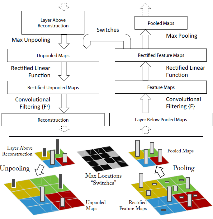
Figure 1. Top: A deconvnet layer (left) attached to a con-vnet layer (right). The deconvnet will reconstruct an approximate version of the convnet features from the layer beneath. Bottom: An illustration of the unpooling operation in the deconvnet, using switches which record the location of the local max in each pooling region (colored zones) during pooling in the convnet.

向caffe中加入新层

2017年4月20日更新：
如何在caffe中增加新的layer
新版的caffe中增加新的layer，变得轻松多了，概括说来，分四步：

1. 在./src/caffe/proto/caffe.proto 中增加 对应layer的paramter message；

2. 在./include/caffe/layers目录下增加该layer的类的声明

3. 在./src/caffe/layers/目录下新建.cpp和.cu文件，进行类实现。

4. 在./src/caffe/gtest/中增加layer的测试代码，对所写的layer前传和反传进行测试，测试还包括速度。

最后一步很多人省了，或者没意识到，但是为保证代码正确，建议还是严格进行测试，磨刀不误砍柴功。
摘自：如何在caffe中增加layer以及caffe中triplet loss layer的实现

GitHub - piergiaj/caffe-deconvnet: A deconvolutional network in caffe中给出了这篇文章的一个开源实现。可以看到源码中只给出了新增的三个层：

1. PoolingSwitches：替代原Pooling层，输出Pool后的结果和最大值的索引位置Switches。
2. SliceHalf：对PoolingSwitches层的结果进行分割，是特殊的Slice层。
3. InvPooling：Pooling的反向操作。

但是由于caffe 版本的原因不能直接将新层加入到caffe工程中，需要做些改动。

1. 改动1：三个层的头文件写在common_layers.hpp和vision_layers.hpp中，这是老版本caffe的写法，新版中需要独立建立对应的头文件，从原文件中拷贝出对应的内容，cpp文件也需要参照新版写法稍微改动下。
2. 改动2：layer_factory.hpp中加入新层的工厂函数（不能粘贴替换！）。
3. 改动3：修改caffe.proto文件中V1LayerParameter。

最后重新编译caffe。

测试

直接使用了github上下载测试用例。convnet使用的是修改后的bvlc_reference_caffenet，将其中的Pooling层换成了PoolingSwitches层。deconvnet是前者的反向操作。二者共享参数。
ConvNet:

DeConvNet:

测试代码如下：

import numpy as np
import matplotlib.pyplot as plt
import os
import sys
sys.path.append('./python')
import caffe

caffe.set_mode_cpu()
net = caffe.Net('python-demo/deploy.prototxt',
                'models/bvlc_reference_caffenet/bvlc_reference_caffenet.caffemodel',
                caffe.TEST)

invnet = caffe.Net('python-demo/invdeploy.prototxt',caffe.TEST)

# input preprocessing: 'data' is the name of the input blob == net.inputs[0]
transformer = caffe.io.Transformer({'data': net.blobs['data'].data.shape})
transformer.set_transpose('data', (2,0,1))
transformer.set_mean('data', np.load('python/caffe/imagenet/ilsvrc_2012_mean.npy').mean(1).mean(1)) # mean pixel
transformer.set_raw_scale('data', 255)  # the reference model operates on images in [0,255] range instead of [0,1]
transformer.set_channel_swap('data', (2,1,0))  # the reference model has channels in BGR order instead of RGB

def norm(x, s=1.0):
    x -= x.min()
    x /= x.max()
    return x*s
#对特征图进行可视化
def vis_square(data, padsize=1, padval=0):
    data -= data.min()
    data /= data.max()

    # force the number of filters to be square
    n = int(np.ceil(np.sqrt(data.shape[0])))
    padding = ((0, n ** 2 - data.shape[0]), (0, padsize), (0, padsize)) + ((0, 0),) * (data.ndim - 3)
    data = np.pad(data, padding, mode='constant', constant_values=(padval, padval))

    # tile the filters into an image
    data = data.reshape((n, n) + data.shape[1:]).transpose((0, 2, 1, 3) + tuple(range(4, data.ndim + 1)))
    data = data.reshape((n * data.shape[1], n * data.shape[3]) + data.shape[4:])
    plt.axis('off')
    plt.imshow(data)


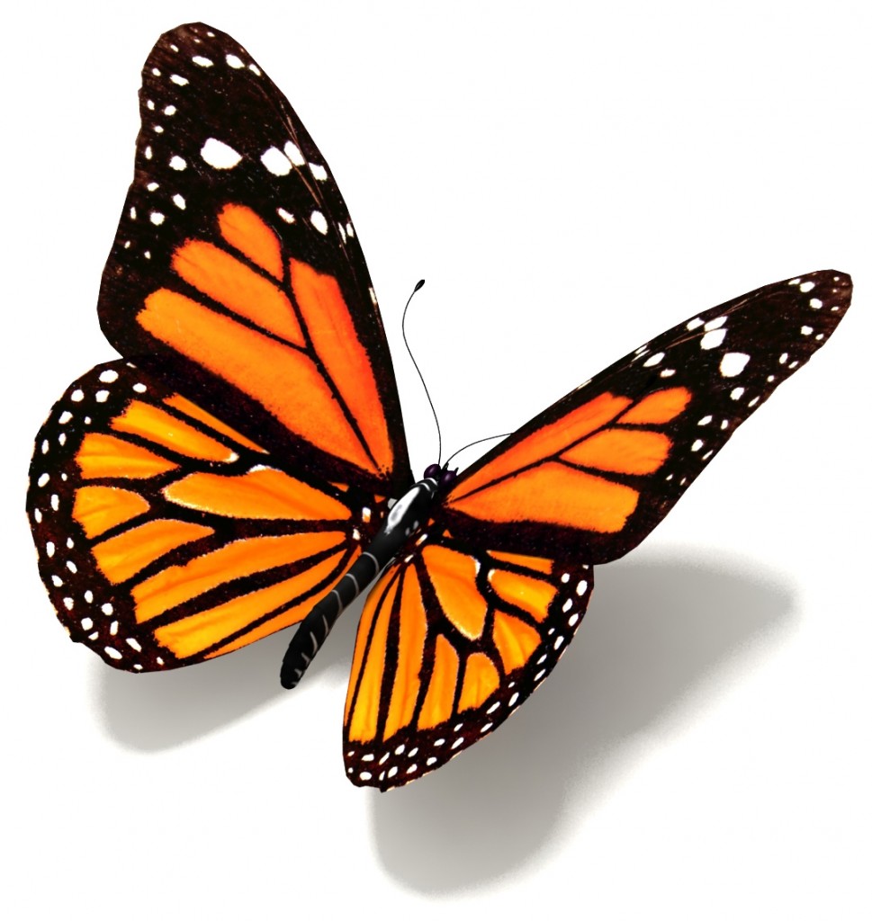
net.blobs['data'].data[...] = transformer.preprocess('data', caffe.io.load_image('test/butterfly.jpg'))
out = net.forward()
#参数共享
for b in invnet.params:
    invnet.params[b][0].data[...] = net.params[b][0].data.reshape(invnet.params[b][0].data.shape)


feat = net.blobs['pool5'].data
feat[0][feat[0] < 0] = 0
vis_square(feat[0], padval=1)
plt.show()


#相关赋值操作
invnet.blobs['pooled'].data[...] = feat
invnet.blobs['switches5'].data[...] = net.blobs['switches5'].data
invnet.blobs['switches2'].data[...] = net.blobs['switches2'].data
invnet.blobs['switches1'].data[...] = net.blobs['switches1'].data
invnet.forward()


plt.clf()
feat = norm(invnet.blobs['conv1'].data[0],255.0)
gci=plt.imshow(transformer.deprocess('data', feat))
plt.colorbar(gci);
plt.show()

输入图像：

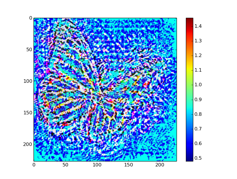
从Conv5层的激活值开始，反卷积结果：