Python 中的Pandas库_python fastparquet column name must be a string.-CSDN博客

http://blog.csdn.net/jiandanjinxin/article/details/70835495

Data Analysis with Python and Pandas Tutorial Introduction

numpy是序列化的矩阵或者序列

pandas是字典形式的numpy，可给不同行列进行重新命名

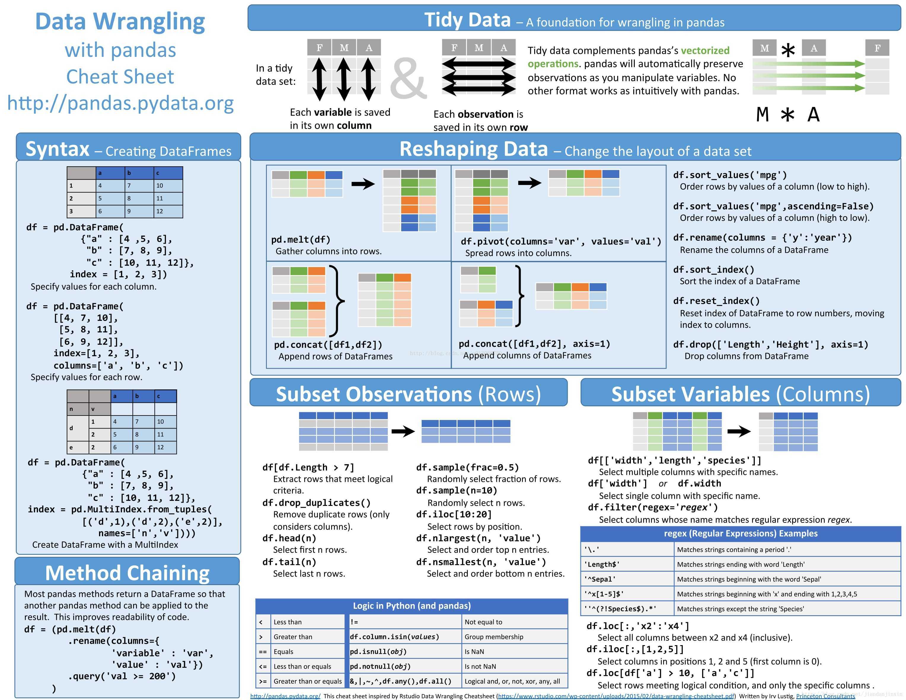
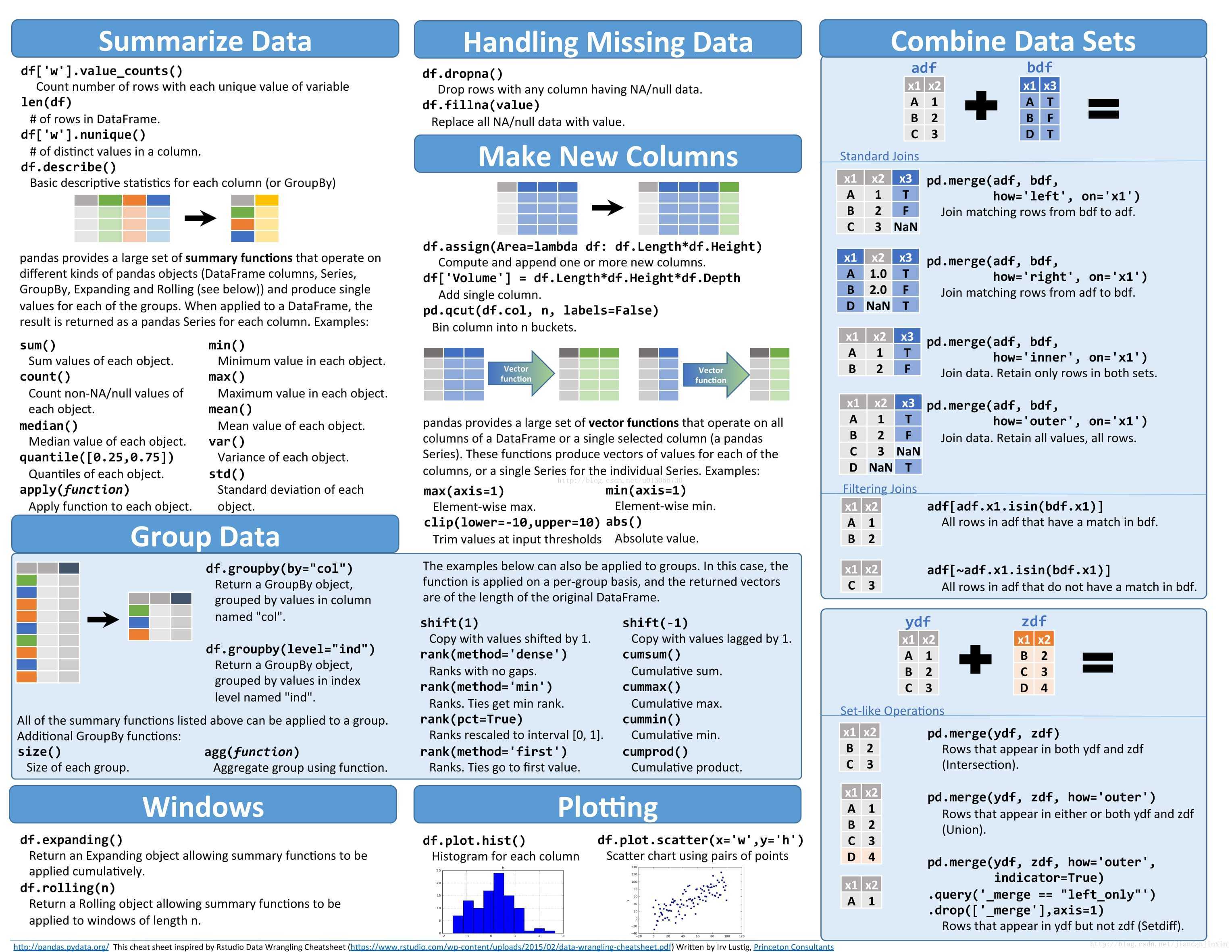
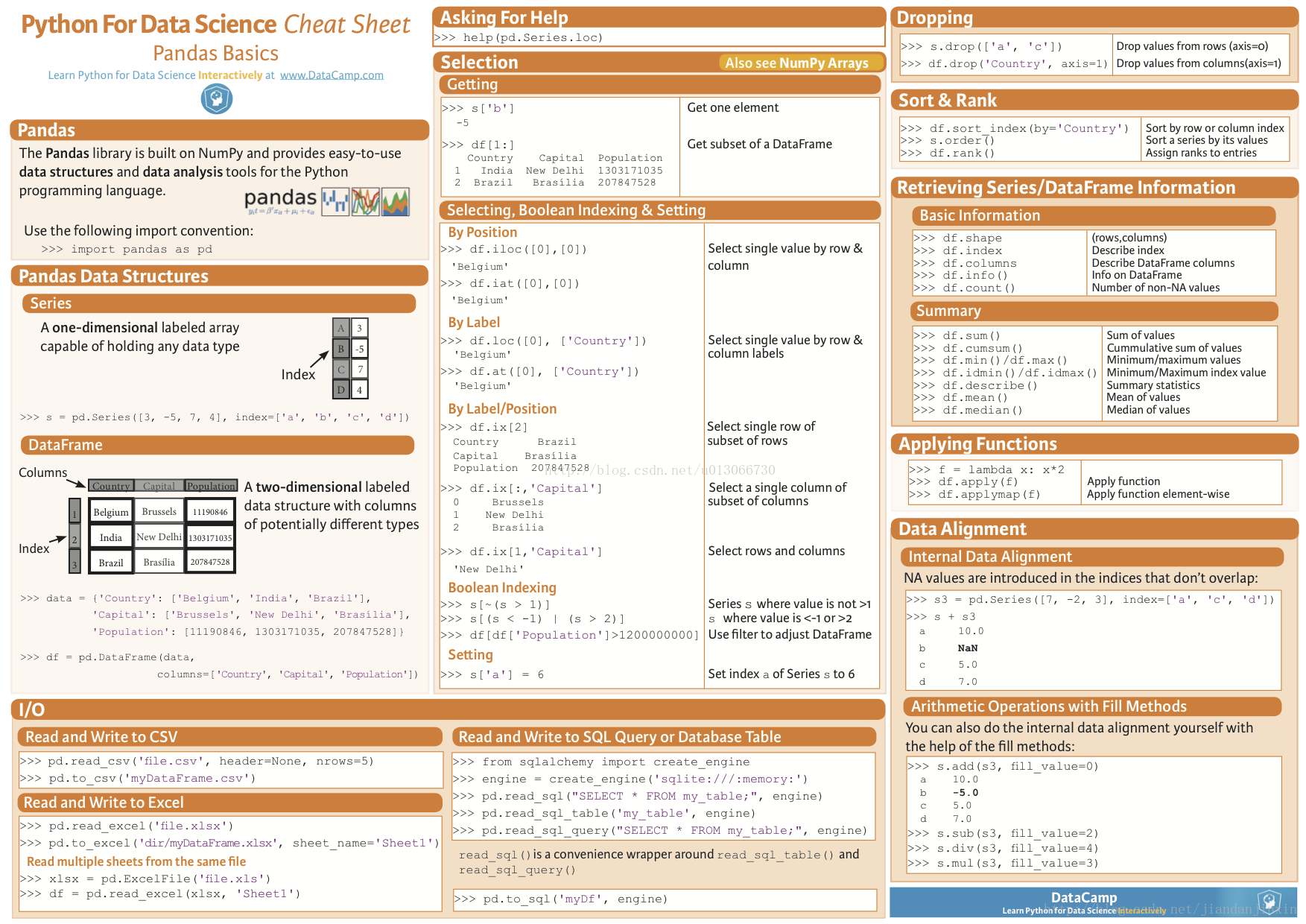
Pandas 小抄

1. Reading and Writing Data

import pandas as pd
#a. Reading a csv file
df=pd.read_csv('Analysis.cav')
#b. Writing content of data frame to csv file
df.to_csv('werfer.csv')
# c.Reading an Excel file
df=pd.read_excel('sdfsdgsd.xlsx', 'sheeet1')
#d. Writing content of data frame to Excel file
df.to_excel('sddg.xlsx', sheet_name='sheet2')
 
 1
2
3
4
5
6
7
8
9
 
 1
2
3
4
5
6
7
8
9

# pandas 导入导出，读取和储存

# The pandas I/O API is a set of top level reader functions accessed like 
# pd.read_csv() that pandas object.

# read_csv  # excel files
# read_excel
# read_hdf
# read_sql
# read_json
# read_msgpack(experimental)
# read_html
# read_gbq(experimental)
# read_stata
# read_sas
# read_clipboard
# read_pickle #自带的亚索

# The corresponding writer functions are object methods that are accessed like
# df.to_csv

# to_csv
# to_excel
# to_hdf
# to_sql
# to_json
# to_msgpack
# to_html
# to_gbq
# to_stata
# to_clipboard
# to_pickle


import pandas as pd

data = pd.read_csv('student.csv')
print(data)

data.to_packle('student.pickle')
 
 1
2
3
4
5
6
7
8
9
10
11
12
13
14
15
16
17
18
19
20
21
22
23
24
25
26
27
28
29
30
31
32
33
34
35
36
37
38
39
40
 
 1
2
3
4
5
6
7
8
9
10
11
12
13
14
15
16
17
18
19
20
21
22
23
24
25
26
27
28
29
30
31
32
33
34
35
36
37
38
39
40

2. Getting Preview of Dataframe

#a.Looking at top n record
df.head(5)
#b.Looking at bottom n record
df.tail(5)
#c.View columns name
df.columns
 
 1
2
3
4
5
6
 
 1
2
3
4
5
6

————————————————— ***3. Rename Columns of Data Frame***

#a. Rename method helps to rename column of data frame
df2 = df.rename(columns={'old_columnname':'new_columnname'})
#This method will create a new data frame with new column name.
#b.To rename the column of existing data frame, set inplace=True.
df.rename(columns={'old_columnname':'new_columnname'}, inplace=True)
 
 1
2
3
4
5
 
 1
2
3
4
5

————————————————— ***4. Selecting Columns or Rows***

#a. Accessing sub data frames
df[['column1','column2']]
#b.Filtering Records
df[df['column1']>10]
df[(df['column1']>10) & df['column2']==30]
df[(df['column1']>10) | df['column2']==30]
 
 1
2
3
4
5
6
 
 1
2
3
4
5
6

# pandas 数据选择

import pandas as pd
import numpy as np

dates = pd.date_range('20170101',periods=6)
df = pd.DataFrame(np.arange(24).reshape((6,4)),index=dates,columns=['A','B','C','D'])
print(df)

print(df['A'],df.A)

print(df[0:3],df['20170101':'20170104'])

# select by label:loc
print(df.loc['20170102'])

print(df.loc[:,['A','B']])

print(df.loc['20170102',['A','B']])

#select by position:iloc
print(df.iloc[3])
print(df.iloc[3,1])
print(df.iloc[1:3,1:3])
print(df.iloc[[1,3,5],1:3])

#mixed selection:ix
print(df.ix[:3,['A','C']])

# Boolean indexing
print(df)
print(df[df.A>8])

 
 1
2
3
4
5
6
7
8
9
10
11
12
13
14
15
16
17
18
19
20
21
22
23
24
25
26
27
28
29
30
31
32
33
 
 1
2
3
4
5
6
7
8
9
10
11
12
13
14
15
16
17
18
19
20
21
22
23
24
25
26
27
28
29
30
31
32
33

5. Handing Missing Values

This is an inevitale part of dealing wiht data. To overcom this hurdle, use dropna or fillna function

#a. dropna: It is used to drop rows or columns having missing data
df1.dropna()
#b.fillna: It is used to fill missing values
df2.fillna(value=5) # It replaces all missing values with 5
mean = df2['column1'].mean()
df2['column1'].fillna(mean) # It replaces all missing values of column1 with mean of available values
 
 1
2
3
4
5
6
 
 1
2
3
4
5
6

————-

from pandas import Series,DataFrame
import pandas as pd
ser = Series([4.5,7.2,-5.3,3.6],index=['d','b','a','c'])
ser
ser.drop('c')
ser
 
 1
2
3
4
5
6
 
 1
2
3
4
5
6

.drop() 返回的是一个新对象，元对象不会被改变。

from pandas import Series,DataFrame
import pandas as pd
import numpy as np

df = pd.DataFrame([[np.nan, 2, np.nan, 0], [3, 4, np.nan, 1],
...                    [np.nan, np.nan, np.nan, 5]],
...                   columns=list('ABCD'))

df

#Drop the columns where all elements are nan
df.dropna(axis=1, how='all')
     A    B  D
0  NaN  2.0  0
1  3.0  4.0  1
2  NaN  NaN  5

#Drop the columns where any of the elements is nan

>>> df.dropna(axis=1, how='any')
   D
0  0
1  1
2  5

#Drop the rows where all of the elements are nan (there is no row to drop, so df #stays the same):

>>> df.dropna(axis=0, how='all')
     A    B   C  D
0  NaN  2.0 NaN  0
1  3.0  4.0 NaN  1
2  NaN  NaN NaN  5

#Drop the rows where any of the elements are nan 

>>> df.dropna(axis=0, how='any')
Empty DataFrame
Columns: [A, B, C, D]
Index: []

#Keep only the rows with at least 2 non-na values:

>>> df.dropna(thresh=2)
     A    B   C  D
0  NaN  2.0 NaN  0
1  3.0  4.0 NaN  1


#Drop where all of the elements are nan, the default is the row, (there is no row to drop, so df #stays the same):

>>> df.dropna(how='all')
     A    B   C  D
0  NaN  2.0 NaN  0
1  3.0  4.0 NaN  1
2  NaN  NaN NaN  5

#Drop  where any of the elements are nan, default is the row 

>>> df.dropna( how='any')
Empty DataFrame
Columns: [A, B, C, D]
Index: []



dfnew = pd.DataFrame([[3435234, 2, 5666, 0], [3, 4, np.nan, 1],
    ...: ...                    [np.nan, np.nan, np.nan, 5]],
    ...: ...                   columns=list('ABCD'))

dfnew.dropna()   #默认对row 进行操作，去掉Na项
         A  B     C  D
0  3435234  2  5666  0

 
 1
2
3
4
5
6
7
8
9
10
11
12
13
14
15
16
17
18
19
20
21
22
23
24
25
26
27
28
29
30
31
32
33
34
35
36
37
38
39
40
41
42
43
44
45
46
47
48
49
50
51
52
53
54
55
56
57
58
59
60
61
62
63
64
65
66
67
68
69
70
71
72
73
 
 1
2
3
4
5
6
7
8
9
10
11
12
13
14
15
16
17
18
19
20
21
22
23
24
25
26
27
28
29
30
31
32
33
34
35
36
37
38
39
40
41
42
43
44
45
46
47
48
49
50
51
52
53
54
55
56
57
58
59
60
61
62
63
64
65
66
67
68
69
70
71
72
73

# 处理丢失数据
import numpy as np
import pandas as pd

dates = pd.date_range('20170101',periods=6)
df = pd.DataFrame(np.arange(24).reshape((6,4)),index=dates,columns=['A','B','C','D'])
print(df)

df.iloc[0,1]=np.nan 
df.iloc[1,2]=np.nan  
print(df.dropna(axis=0,how='any'))#how={'any','all'} default is 'any'
print(df.dropna(axis=1,how='all'))

#填入数据
print(df.fillna(value=0))
#打印缺失数据
print(df.isnull())
#打印出缺失数据，当数据比较大时
print(np.any(df.isnull())==True)

 
 1
2
3
4
5
6
7
8
9
10
11
12
13
14
15
16
17
18
19
20
 
 1
2
3
4
5
6
7
8
9
10
11
12
13
14
15
16
17
18
19
20

6. Creating New Columns

New column is a function of existing columns

df['NewColumn1'] = df['column2'] # Create a copy of existing column2
df['NewColumn2'] = df['column2'] + 10 # Add 10 to existing column2 then create a new one
df['NewColumn3'] = df['column1'] + df['column2'] # Add elements of column1 and column2 then create new column
 
 1
2
3
 
 1
2
3

import pandas as pd 
import numpy as np

s = pd.Series([1,3,5,np.nan,55,2])
print(s)


dates = pd.date_range('20160101',periods=6)
print(dates)

df = pd.DataFrame(np.random.random(6,4),index=dates,columns=['a','b','c','d'])
print(df)

df1 = pd.DataFrame(np.arange(12).reshape((3,4)))
print(df1)

df2 = pd.DataFrame({'A':1.,
    'B':pd.Timestamp('20170101'),
    'C':pd.Series(1,index=list(range(4)),dtype='float32'),
    'D':np.array([3]*4,dtype='int32'),
    'E':pd.Categorical(["test","train,"test","train"]),
        'F':'foo'})

print(df2.dtypes)  
print(df2.columns)
print(df2.values)

print(df2.describe)

print(df2.T)

print(df2.sort_index(axis=1,ascending=False))
df2.sort_values(by='E')

 
 1
2
3
4
5
6
7
8
9
10
11
12
13
14
15
16
17
18
19
20
21
22
23
24
25
26
27
28
29
30
31
32
33
34
 
 1
2
3
4
5
6
7
8
9
10
11
12
13
14
15
16
17
18
19
20
21
22
23
24
25
26
27
28
29
30
31
32
33
34

#添加空行
df['F'] = np.nan 
print(df)

df['E']=pd.Series([1,2,3,4,5,6],index=pd.date_range('20170101',periods=6))
print(df)

 
 1
2
3
4
5
6
7
 
 1
2
3
4
5
6
7

7. Aggregate

a. Groupby: Groupby helps to perform three operations.
i. Splitting the data into groups
ii. Applying a function to each group individually
iii. Combining the result into a data structure

df.groupby('column1').sum()
df.groupby(['column1','column2']).count()
 
 1
2
 
 1
2

b. Pivot Table: It helps to generate data structure. It has three components index, columns and values(similar to excel)

pd.pivot_table(df, values='column1',index=['column2','column3'],columns=['column4'])
 
 1
 
 1

By default, it shows the sum of values column but you can change it using argument aggfunc

pd.pivot_table(df, values='column1',index=['column2','column3'],columns=['column4'], aggfunc=len)
 
 1
 
 1

It shows count c. Cross Tab: Cross Tab computes the simple cross tabulation of two factors

pd.crosstab(df.column1, df.column2)
 
 1
 
 1

————————————————— ***8. Merging /Concatenating DataFrames*** a. Concatenating: It concatenate two or more data frames based on their columns

pd.concat([df1, df2])
 
 1
 
 1

b. Merging: We can perform left, right and inner join also.

pd.merge(df1,df2, on='column1',how='inner')
pd.merge(df1,df2, on='column1',how='left')
pd.merge(df1,df2, on='column1',how='right')
pd.merge(df1,df2, on='column1',how='outer')
 
 1
2
3
4
 
 1
2
3
4

# pandas 合并concat


import pandas as pd
import numpy as np

#concatenating

df1 = pd.DataFrame(np.ones((3,4))*0,columns=['a','b','c','d'])
df2 = pd.DataFrame(np.ones((3,4))*1,columns=['a','b','c','d'])
df3 = pd.DataFrame(np.ones((3,4))*2,columns=['a','b','c','d'])

print(df1)
print(df2)
print(df3)

result = pd.concat([df1,df2,df3],axis=0)#行合并
print(result)
#result1 = pd.concat([df1,df2,df3],axis=1)#列合并
#print(result1)

result = pd.concat([df1,df2,df3],axis=0,ignore_index=True)#行合并,忽略index
print(result)



#join,['inner','outer']
df1 = pd.DataFrame(np.ones((3,4))*0,columns=['a','b','c','d'],index=[1,2,3])
df2 = pd.DataFrame(np.ones((3,4))*1,columns=['a','b','c','d'],index=[2,3,4])
print(df1)
print(df2)

result2 = pd.concat([df1,df2],join='outer'，ignore_index=True)# 补充为na
print(result2)
result22 = pd.concat([df1,df2],join='outer')# 补充为na
print(result22)
result3 = pd.concat([df1,df2],join='inner'，ignore_index=True) # 裁剪掉
print(result3)
result33 = pd.concat([df1,df2],join='inner') # 裁剪掉
print(result33)


#join_axes
df1 = pd.DataFrame(np.ones((3,4))*0,columns=['a','b','c','d'],index=[1,2,3])
df2 = pd.DataFrame(np.ones((3,4))*1,columns=['a','b','c','d'],index=[2,3,4])
res = pd.concat([df1,df2],axis=1,join_axes=[df1.index])
print(res)

res1 = pd.concat([df1,df2],axis=1)
print(res1)


#append
df1 = pd.DataFrame(np.ones((3,4))*0,columns=['a','b','c','d'])
df2 = pd.DataFrame(np.ones((3,4))*1,columns=['a','b','c','d'])
df3 = pd.DataFrame(np.ones((3,4))*1,columns=['a','b','c','d'])
res11 = df1.append(df2,ignore_index=True)
print(res11)
res12 = df1.append([df2,df3],ignore_index=True)
print(res12)

s1 = pd.Series([1,2,3,4],index=['a','b','c','d'])

res13=df1.append(s1,ignore_index=True)
print(res13)


#pandas 合并merge

import pandas as pd

#merging two df by key/keys.(may be used in database)
#simple example
left = pd.DataFrame({'key':['K0','K1','K2','K3'],
                      'A':['A0','A1','A2','A3'],
                      'B':['B0','B1','B2','B3']})
right = pd.DataFrame({'key':['K0','K1','K2','K3'],
                      'C':['C0','C1','C2','C3'],
                      'D':['D0','D1','D2','D3']})

print(lef)
print(right)
res14 = pd.merge(left,right,on='key')
print(res14)


#consider two keys
left = pd.DataFrame({'key1':['K0','K0','K1','K2'],
                     'key2':['K0','K1','K0','K1'],
                      'A':['A0','A1','A2','A3'],
                      'B':['B0','B1','B2','B3']})
right = pd.DataFrame({'key1':['K0','K1','K1','K2'],
                      'key2':['K0','K0','K0','K0'],
                      'C':['C0','C1','C2','C3'],
                      'D':['D0','D1','D2','D3']})
print(left)
print(right)

res15 = pd.merge(left,right,on=['key1','key2'])
print(res15)
#how =['left','right','inner','outer']
res16 = pd.merge(left,right,on=['key1','key2'],how='inner')
print(res16)
 
 1
2
3
4
5
6
7
8
9
10
11
12
13
14
15
16
17
18
19
20
21
22
23
24
25
26
27
28
29
30
31
32
33
34
35
36
37
38
39
40
41
42
43
44
45
46
47
48
49
50
51
52
53
54
55
56
57
58
59
60
61
62
63
64
65
66
67
68
69
70
71
72
73
74
75
76
77
78
79
80
81
82
83
84
85
86
87
88
89
90
91
92
93
94
95
96
97
98
99
100
101
102
103
 
 1
2
3
4
5
6
7
8
9
10
11
12
13
14
15
16
17
18
19
20
21
22
23
24
25
26
27
28
29
30
31
32
33
34
35
36
37
38
39
40
41
42
43
44
45
46
47
48
49
50
51
52
53
54
55
56
57
58
59
60
61
62
63
64
65
66
67
68
69
70
71
72
73
74
75
76
77
78
79
80
81
82
83
84
85
86
87
88
89
90
91
92
93
94
95
96
97
98
99
100
101
102
103

9. Applying function to element, column or dataframe

a. Map: It iterates over each element of a series

df['column1'].map(lambda x: 10+x)  #this will add 10 to each element of column1
df['column2'].map(lambda x:'AV'+x) # this will concatenate 'AV' at the beginning of each element of column2(column format is string)
 
 1
2
 
 1
2

b. Apply: As the name suggests, applies a function along any axis of the DataFrame

df[['column1','column2']].apply(sum) #It will returns the sum of all the values of column1 and column2
 
 1
 
 1

c. ApplyMap: This helps to apply a function to each element of dataframe

func = lambda x: x+2
df.applymap(func) # it will add 2 to each element of dataframe(all columns of dataframe must be numeric type)
 
 1
2
 
 1
2

————————————————— ***10. Identify unique value*** Function unique helps to return unique values of a column

df['Column1'].unique()
 
 1
 
 1

————————————————— ***11. Basic Stats*** Pandas helps to understand the data using basic statistical methods. a. describe: This returns the quick stats(count, mean, std, min, first quartile, median, third quartile, max) on suitable columns

df.describe()
 
 1
 
 1

b. covariance: It returns the co-variance between suitable columns

df.cov()
 
 1
 
 1

c.correlation: It returns the co-variance between suitable columns.

df.corr()
 
 1
 
 1

——— 本文中的 Python-Pandas.ipynb格式见[CSDN下载](http://download.csdn.net/detail/jiandanjinxin/9826981)。

#https://python.freelycode.com/contribution/detail/333
#https://python.freelycode.com/contribution/detail/334
#http://www.datadependence.com/2016/05/scientific-python-pandas/

#Python科学计算之Pandas
#导入Pandas的标准方式
import pandas as pd # This is the standard
 
 1
2
3
4
5
6
7
 
 1
2
3
4
5
6
7

#Pandas的数据类型
#Pandas基于两种数据类型：series与dataframe。
#一个series是一个一维的数据类型，其中每一个元素都有一个标签。
#series类似于Numpy中元素带标签的数组。其中，标签可以是数字或者字符串。
#一个dataframe是一个二维的表结构。Pandas的dataframe可以存储许多种不同的数据类型，并且每一个坐标轴都有自己的标签。
#你可以把它想象成一个series的字典项。
 
 1
2
3
4
5
6
 
 1
2
3
4
5
6

#将数据导入Pandas,采用[英国政府数据中关于降雨量数据](https://data.gov.uk/dataset/average-temperature-and-rainfall-england-and-wales/resource/3fea0f7b-5304-4f11-a809-159f4558e7da)
# Reading a csv into Pandas,从csv文件中读取到了数据，并将他们存入了dataframe中
#header关键字告诉Pandas这些数据是否有列名，在哪里。如果没有列名，你可以将其置为None。
df = pd.read_csv('uk_rain_2014.csv', header=0)
 
 1
2
3
4
 
 1
2
3
4

#将你的数据准备好以进行挖掘和分析
#想要快速查看前x行数据
#Getting first x rows
df.head(5)
 
 1
2
3
4
 
 1
2
3
4

	Water Year	Rain (mm) Oct-Sep	Outflow (m3/s) Oct-Sep	Rain (mm) Dec-Feb	Outflow (m3/s) Dec-Feb	Rain (mm) Jun-Aug	Outflow (m3/s) Jun-Aug
0	1980/81	1182	5408	292	7248	174	2212
1	1981/82	1098	5112	257	7316	242	1936
2	1982/83	1156	5701	330	8567	124	1802
3	1983/84	993	4265	391	8905	141	1078
4	1984/85	1182	5364	217	5813	343	4313

#想要获得最后x行的数据
#Getting last x rows
#Pandas不是从dataframe的结尾处开始倒着输出数据，
#而是按照它们在dataframe中固有的顺序输出给你。
df.tail(5)
 
 1
2
3
4
5
 
 1
2
3
4
5

	Water Year	Rain (mm) Oct-Sep	Outflow (m3/s) Oct-Sep	Rain (mm) Dec-Feb	Outflow (m3/s) Dec-Feb	Rain (mm) Jun-Aug	Outflow (m3/s) Jun-Aug
28	2008/09	1139	4941	268	6690	323	3189
29	2009/10	1103	4738	255	6435	244	1958
30	2010/11	1053	4521	265	6593	267	2885
31	2011/12	1285	5500	339	7630	379	5261
32	2012/13	1090	5329	350	9615	187	1797

df.columns
 
 1
 
 1

Index([’Water Year’, ‘Rain (mm) Oct-Sep’, ‘Outflow (m3/s) Oct-Sep’, ‘Rain (mm) Dec-Feb’, ‘Outflow (m3/s) Dec-Feb’, ‘Rain (mm) Jun-Aug’, ‘Outflow (m3/s) Jun-Aug’], dtype=’object’)

#Changing column labels.
df.columns = ['water_year', 'rain_octsep', 'outflow_octsep', 'rain_decfeb', 'outflow_decfeb', 'rain_junaug', 'outflow_junaug']
df.head(5)
 
 1
2
3
 
 1
2
3

	water_year	rain_octsep	outflow_octsep	rain_decfeb	outflow_decfeb	rain_junaug	outflow_junaug
0	1980/81	1182	5408	292	7248	174	2212
1	1981/82	1098	5112	257	7316	242	1936
2	1982/83	1156	5701	330	8567	124	1802
3	1983/84	993	4265	391	8905	141	1078
4	1984/85	1182	5364	217	5813	343	4313

#取数据的行数，即条目数
#Finding out how many rows dataset has.
len(df)
 
 1
2
3
 
 1
2
3

#数据的一些基本的统计信息
#Finding out basic statistical information on your dataset.
pd.options.display.float_format = '{:,.3f}'.format
#Limit output to 3 decimal places.计数，均值，标准方差
df.describe()
 
 1
2
3
4
5
 
 1
2
3
4
5

	rain_octsep	outflow_octsep	rain_decfeb	outflow_decfeb	rain_junaug	outflow_junaug
count	33.000	33.000	33.000	33.000	33.000	33.000
mean	1,129.000	5,019.182	325.364	7,926.545	237.485	2,439.758
std	101.900	658.588	69.995	1,692.800	66.168	1,025.914
min	856.000	3,479.000	206.000	4,578.000	103.000	1,078.000
25%	1,053.000	4,506.000	268.000	6,690.000	193.000	1,797.000
50%	1,139.000	5,112.000	309.000	7,630.000	229.000	2,142.000
75%	1,182.000	5,497.000	360.000	8,905.000	280.000	2,959.000
max	1,387.000	6,391.000	484.000	11,486.000	379.000	5,261.000

#过滤
#提取一整列。可以直接使用列标签
#Getting a column by label
df['rain_octsep']
 
 1
2
3
4
 
 1
2
3
4

0 1182 1 1098 2 1156 3 993 4 1182 5 1027 6 1151 7 1210 8 976 9 1130 10 1022 11 1151 12 1130 13 1162 14 1110 15 856 16 1047 17 1169 18 1268 19 1204 20 1239 21 1185 22 1021 23 1165 24 1095 25 1046 26 1387 27 1225 28 1139 29 1103 30 1053 31 1285 32 1090 Name: rain_octsep, dtype: int64

#不使用空格和横线等可以让我们以访问类属性相同的方法来访问列，即使用点运算符
#Getting a column by label using.
df.rain_octsep
 
 1
2
3
 
 1
2
3

#boolean masking
#Creating a series of booleans based on a conditional
df.rain_octsep <1000 
df['rain_octsep'] <1000
 
 1
2
3
4
 
 1
2
3
4

0 False 1 False 2 False 3 True 4 False 5 False 6 False 7 False 8 True 9 False 10 False 11 False 12 False 13 False 14 False 15 True 16 False 17 False 18 False 19 False 20 False 21 False 22 False 23 False 24 False 25 False 26 False 27 False 28 False 29 False 30 False 31 False 32 False Name: rain_octsep, dtype: bool

#使用多条条件表达式来进行过滤
#Filtering by multiple conditionals
#将返回rain_octsep小于1000并且outflow_octsep小于4000的那些条目。
df[(df.rain_octsep <1000) & (df.outflow_octsep <4000)]
# Can't use the keyword 'and'
 
 1
2
3
4
5
 
 1
2
3
4
5

	water_year	rain_octsep	outflow_octsep	rain_decfeb	outflow_decfeb	rain_junaug	outflow_junaug
15	1995/96	856	3479	245	5515	172	1439

#数据中有字符串，也可以使用字符串方法来过滤数据。
#必须使用.str.[string method]，你不能直接在字符串上直接调用字符串方法。
#Filtering by string methods
df[df.water_year.str.startswith('199')] #这一语句返回1990年代的所有条目
 
 1
2
3
4
 
 1
2
3
4

	water_year	rain_octsep	outflow_octsep	rain_decfeb	outflow_decfeb	rain_junaug	outflow_junaug
10	1990/91	1022	4418	305	7120	216	1923
11	1991/92	1151	4506	246	5493	280	2118
12	1992/93	1130	5246	308	8751	219	2551
13	1993/94	1162	5583	422	10109	193	1638
14	1994/95	1110	5370	484	11486	103	1231
15	1995/96	856	3479	245	5515	172	1439
16	1996/97	1047	4019	258	5770	256	2102
17	1997/98	1169	4953	341	7747	285	3206
18	1998/99	1268	5824	360	8771	225	2240
19	1999/00	1204	5665	417	10021	197	2166

#索引
#如果行有数字索引，可以使用iloc引用他们
#Getting a row via a numerical index
#iloc仅仅作用于数字索引。它将会返回该行的一个series。
df.iloc[30]
 
 1
2
3
4
5
 
 1
2
3
4
5

water_year 2010/11 rain_octsep 1053 outflow_octsep 4521 rain_decfeb 265 outflow_decfeb 6593 rain_junaug 267 outflow_junaug 2885 Name: 30, dtype: object

#可能在数据集里有年份的列，或者年代的列
#Setting a new index from an existing column
df = df.set_index(['water_year'])
df.head(5)
 
 1
2
3
4
 
 1
2
3
4

	rain_octsep	outflow_octsep	rain_decfeb	outflow_decfeb	rain_junaug	outflow_junaug
water_year
1980/81	1182	5408	292	7248	174	2212
1981/82	1098	5112	257	7316	242	1936
1982/83	1156	5701	330	8567	124	1802
1983/84	993	4265	391	8905	141	1078
1984/85	1182	5364	217	5813	343	4313

#在上面这个例子中，我们把我们的索引值全部设置为了字符串。这意味着我们不可以使用iloc索引这些列了。
#这种情况该如何？我们使用loc。
#Getting a row via a label-based index
df.loc['2000/01']  
#这里，loc和iloc一样会返回你所索引的行数据的一个series。
#唯一的不同是此时你使用的是字符串标签进行引用，而不是数字标签。
 
 1
2
3
4
5
6
 
 1
2
3
4
5
6

rain_octsep 1239 outflow_octsep 6092 rain_decfeb 328 outflow_decfeb 9347 rain_junaug 236 outflow_junaug 2142 Name: 2000/01, dtype: int64

#如果loc是字符串标签的索引方法，iloc是数字标签的索引方法，那什么是ix呢？
#事实上，ix是一个字符串标签的索引方法，但是它同样支持数字标签索引作为它的备选。
#Getting a row via a label-based or numerical index
df.ix['1999/00'] # Label based with numerical index fallback * Not recommend
#正如loc和iloc，上述代码将返回一个series包含你所索引的行的数据
 
 1
2
3
4
5
 
 1
2
3
4
5

rain_octsep 1204 outflow_octsep 5665 rain_decfeb 417 outflow_decfeb 10021 rain_junaug 197 outflow_junaug 2166 Name: 1999/00, dtype: int64

#既然ix可以完成loc和iloc二者的工作，为什么还需要它们呢?
#最主要的原因是ix有一些轻微的不可预测性。还记得我说数字标签索引是ix的备选吗？
#数字标签可能会让ix做出一些奇怪的事情，例如将一个数字解释成一个位置。
#而loc和iloc则为你带来了安全的、可预测的、内心的宁静。
#然而必须指出的是，ix要比loc和iloc更快。
 
 1
2
3
4
5
 
 1
2
3
4
5

#调用sort_index来对dataframe实现排序
#inplace=True to apple the sorting in place
#置了关键字参数’ascending’为False。这样，我的数据会以降序排列
df.sort_index(ascending=False).head(5)
 
 1
2
3
4
 
 1
2
3
4

	rain_octsep	outflow_octsep	rain_decfeb	outflow_decfeb	rain_junaug	outflow_junaug
water_year
2012/13	1090	5329	350	9615	187	1797
2011/12	1285	5500	339	7630	379	5261
2010/11	1053	4521	265	6593	267	2885
2009/10	1103	4738	255	6435	244	1958
2008/09	1139	4941	268	6690	323	3189

#当你为一列数据设置了一个索引时，它们将不再是数据本身了。
#如果你想把索引设置为原始数据的形式，
#你可以使用和set_index相反的操作——reset_index。
#Returning an index to data
#这将返回数据原始的索引形式。
df = df.reset_index('water_year')
df.head(5)
 
 1
2
3
4
5
6
7
 
 1
2
3
4
5
6
7

	water_year	rain_octsep	outflow_octsep	rain_decfeb	outflow_decfeb	rain_junaug	outflow_junaug
0	1980/81	1182	5408	292	7248	174	2212
1	1981/82	1098	5112	257	7316	242	1936
2	1982/83	1156	5701	330	8567	124	1802
3	1983/84	993	4265	391	8905	141	1078
4	1984/85	1182	5364	217	5813	343	4313

#对数据集应用函数
#Applying a function to a column
def base_year(year):
    base_year = year[:4]
    base_year = pd.to_datetime(base_year).year
    return base_year

df['year'] = df.water_year.apply(base_year)
df.head(5)
 
 1
2
3
4
5
6
7
8
9
 
 1
2
3
4
5
6
7
8
9

	water_year	rain_octsep	outflow_octsep	rain_decfeb	outflow_decfeb	rain_junaug	outflow_junaug	year
0	1980/81	1182	5408	292	7248	174	2212	1980
1	1981/82	1098	5112	257	7316	242	1936	1981
2	1982/83	1156	5701	330	8567	124	1802	1982
3	1983/84	993	4265	391	8905	141	1078	1983
4	1984/85	1182	5364	217	5813	343	4313	1984

#使用apply的方法，即如何对一列应用一个函数。
#如果你想对整个数据集应用某个函数，你可以使用dataset.applymap()。
 
 1
2
 
 1
2

#操作一个数据集结构
#另一件经常会对dataframe所做的操作是为了让它们呈现出一种更便于使用的形式而对它们进行的重构。
#Manipulating structure (groupby,unstack,pivot)
#Groupby
df.groupby(df.year // 10*10).max()
 
 1
2
3
4
5
 
 1
2
3
4
5

	water_year	rain_octsep	outflow_octsep	rain_decfeb	outflow_decfeb	rain_junaug	outflow_junaug	year
year
1980	1989/90	1210	5701	470	10520	343	4313	1989
1990	1999/00	1268	5824	484	11486	285	3206	1999
2000	2009/10	1387	6391	437	10926	357	5168	2009
2010	2012/13	1285	5500	350	9615	379	5261	2012

#对多行进行分组操作
#Grouping by multiple columns
decade_rain = df.groupby([df.year // 10*10,
                         df.rain_octsep // 1000*1000])[['outflow_octsep',
                                                       'outflow_decfeb','outflow_junaug']].mean()
decade_rain
 
 1
2
3
4
5
6
 
 1
2
3
4
5
6

		outflow_octsep	outflow_decfeb	outflow_junaug
year	rain_octsep
1980	0	4,297.500	7,685.000	1,259.000
1980	1000	5,289.625	7,933.000	2,572.250
1990	0	3,479.000	5,515.000	1,439.000
1990	1000	5,064.889	8,363.111	2,130.556
2000	1000	5,030.800	7,812.100	2,685.900
2010	1000	5,116.667	7,946.000	3,314.333

#unstack操作的功能是将某一列前置成为列标签。
#Unstacking
decade_rain.unstack(0)
#它将标识‘year’索引的第0列推起来，变为了列标签。
 
 1
2
3
4
 
 1
2
3
4

	outflow_octsep				outflow_decfeb				outflow_junaug
year	1980	1990	2000	2010	1980	1990	2000	2010	1980	1990	2000	2010
rain_octsep
0	4,297.500	3,479.000	nan	nan	7,685.000	5,515.000	nan	nan	1,259.000	1,439.000	nan	nan
1000	5,289.625	5,064.889	5,030.800	5,116.667	7,933.000	8,363.111	7,812.100	7,946.000	2,572.250	2,130.556	2,685.900	3,314.333

#再附加一个unstack操作。这次我们对’rain_octsep’索引的第1列操作：
#More unstacking
decade_rain.unstack(1)
 
 1
2
3
 
 1
2
3

	outflow_octsep		outflow_decfeb		outflow_junaug
rain_octsep	0	1000	0	1000	0	1000
year
1980	4,297.500	5,289.625	7,685.000	7,933.000	1,259.000	2,572.250
1990	3,479.000	5,064.889	5,515.000	8,363.111	1,439.000	2,130.556
2000	nan	5,030.800	nan	7,812.100	nan	2,685.900
2010	nan	5,116.667	nan	7,946.000	nan	3,314.333

#创造一个新的dataframe
#Create a new dataframe containing entries which has rain_octsep values of
#greater than 1250
high_rain = df[df.rain_octsep > 1250]
high_rain
 
 1
2
3
4
5
 
 1
2
3
4
5

	water_year	rain_octsep	outflow_octsep	rain_decfeb	outflow_decfeb	rain_junaug	outflow_junaug	year
18	1998/99	1268	5824	360	8771	225	2240	1998
26	2006/07	1387	6391	437	10926	357	5168	2006
31	2011/12	1285	5500	339	7630	379	5261	2011

#上述代码为我们创建了如下的dataframe，我们将对它进行pivot操作
#ivot实际上是在本文中我们已经见过的操作的组合。
#首先，它设置了一个新的索引(set_index())，然后它对这个索引排序(sort_index())，最后它会进行unstack操作。
#组合起来就是一个pivot操作。看看你能不能想想会发生什么：
#Pivoting
#does set_index,sort_index and unstack in a row
high_rain.pivot('year', 'rain_octsep')[['outflow_octsep',
                                       'outflow_decfeb','outflow_junaug']].fillna('')
 
 1
2
3
4
5
6
7
8
 
 1
2
3
4
5
6
7
8

	outflow_octsep			outflow_decfeb			outflow_junaug
rain_octsep	1268	1285	1387	1268	1285	1387	1268	1285	1387
year
1998	5,824.000			8,771.000			2,240.000
2006			6,391.000			10,926.000			5,168.000
2011		5,500.000			7,630.000			5,261.000

#合并数据集
#有时候你有两个单独的数据集，它们直接互相关联，而你想要比较它们的差异或者合并它们
#Merging two datasets together
rain_jpn = pd.read_csv('jpn_rain.csv')
rain_jpn.column = ['year', 'jpn_rainfall']
uk_jpn_rain = df.merge(rain_jpn, on = 'year')
uk_jpn_rain.head(5)
#可以看到，两个数据集在年份这一类上已经合并了。rain_jpn数据集仅仅包含年份以及降雨量。
 
 1
2
3
4
5
6
7
8
 
 1
2
3
4
5
6
7
8

#采用Pandas快速绘制图表
#Using pandas to quickly plot graphs
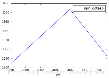
%matplotlib inline
high_rain.plot(x='year', y='rain_octsep')
 
 1
2
3
4
 
 1
2
3
4

<matplotlib.axes._subplots.AxesSubplot at 0x7f1214a5d748>

这里写图片描述

#存储你的数据集
#Saving your data to a csv
df.to_csv('high_rain.csv')
 
 1
2
3
 
 1
2
3

# pandas plot
import pandas as pd
import numpy as np
import matplotlib.pyplot as plt 

#plot data

# Series
data = pd.Series(np.random.randn(1000),index=np.arange(1000))
data = data.cumsum()
data.plot()
plt.show()
plt.plot(x= , y = )

#DataFrame
data = pd.DataFrame(np.random.randn(1000,4),
                 index=np.arange(1000),
                 columns=list("ABCD"))
data =data.cumsum()
print(data.head())
data.plot()
plt.show()

#plot methods:
#'bar','hist','box','area','scatter','hexbin','pie'
data.plot.scatter(x='A',y='B',color='DarkBlue',label='Class1')
data.plot.scatter(x='A',y='C',color='DarkGreen',lable='Class2',ax=ax)
plt.show()

 
 1
2
3
4
5
6
7
8
9
10
11
12
13
14
15
16
17
18
19
20
21
22
23
24
25
26
27
28
29
 
 1
2
3
4
5
6
7
8
9
10
11
12
13
14
15
16
17
18
19
20
21
22
23
24
25
26
27
28
29