【Seaborn】sns.lmplot() 函数：多类别回归拟合散点图

sns.lmplot() —— 多类别回归拟合散点图（Linear Model Plot）

seaborn.lmplot() 是 回归分析的可视化工具，它与 sns.regplot() 类似，但支持按类别 (hue) 区分数据，适用于 分组回归分析。

---

1. 语法

import seaborn as sns

sns.lmplot(data=None, x=None, y=None, hue=None, col=None, row=None, scatter=True, fit_reg=True, ci=95)

主要参数

参数	作用
data	DataFrame 数据集
x	X 轴变量（数值）
y	Y 轴变量（数值）
hue	按类别分色
col / row	生成 多个子图
scatter	是否绘制散点（默认 True）
fit_reg	是否绘制回归线（默认 True）
ci	置信区间（默认 95%）

---

2. 基本用法

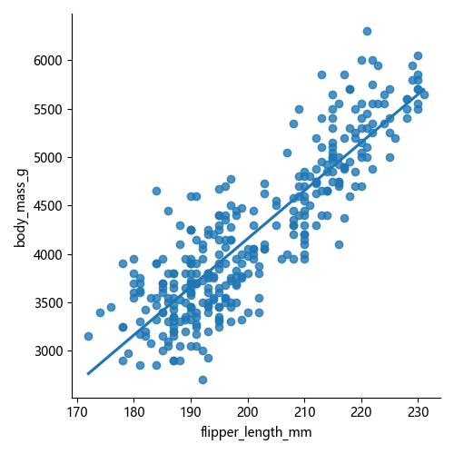
2.1 画回归拟合散点图

import seaborn as sns
import matplotlib.pyplot as plt

# 加载数据
data = sns.load_dataset("penguins")

# 绘制回归拟合散点图
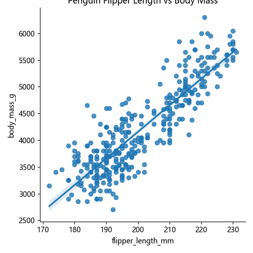
sns.lmplot(data=data, x="flipper_length_mm", y="body_mass_g")

plt.title("Penguin Flipper Length vs Body Mass")
plt.show()

📌 说明

• x="flipper_length_mm" → 企鹅的鳍长。
• y="body_mass_g" → 企鹅体重。
• 蓝色阴影区域 是 95% 置信区间。
  

---

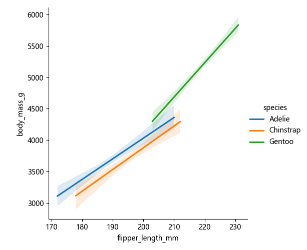
2.2 按类别着色（hue 参数）

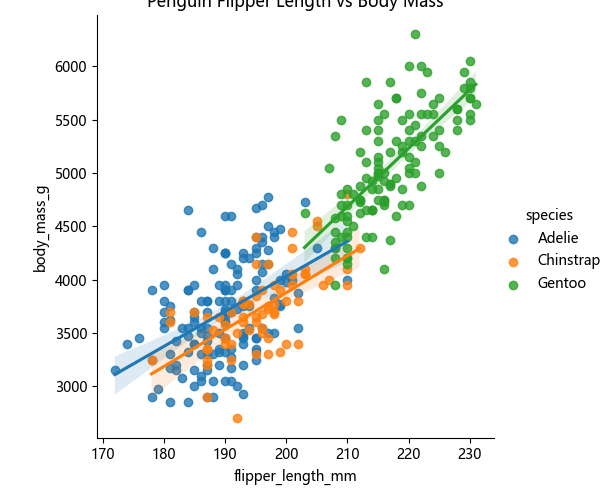
sns.lmplot(data=data, x="flipper_length_mm", y="body_mass_g", hue="species")

plt.show()

📌 作用

• hue="species" → 不同种类用不同颜色表示。
• 每种类别都有自己的回归线。
  

---

3. 多子图（col 和 row）

3.1 按列 (col) 拆分

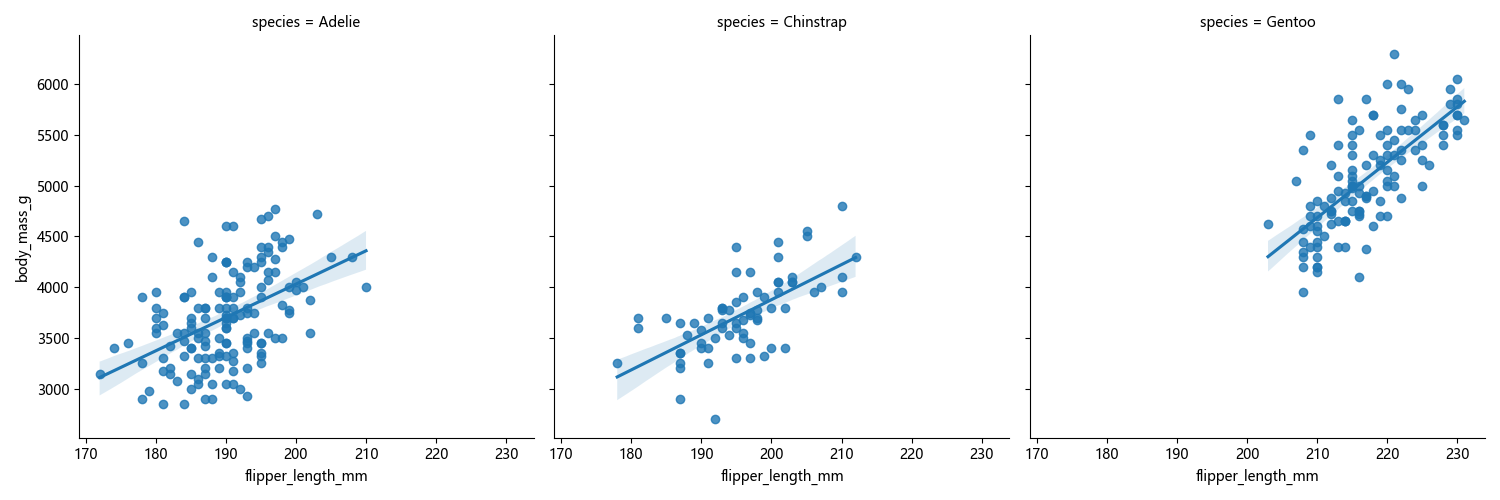
sns.lmplot(data=data, x="flipper_length_mm", y="body_mass_g", col="species")

plt.show()

📌 作用

• col="species" → 每个物种单独绘制回归图。
  

---

3.2 按行 (row) 拆分

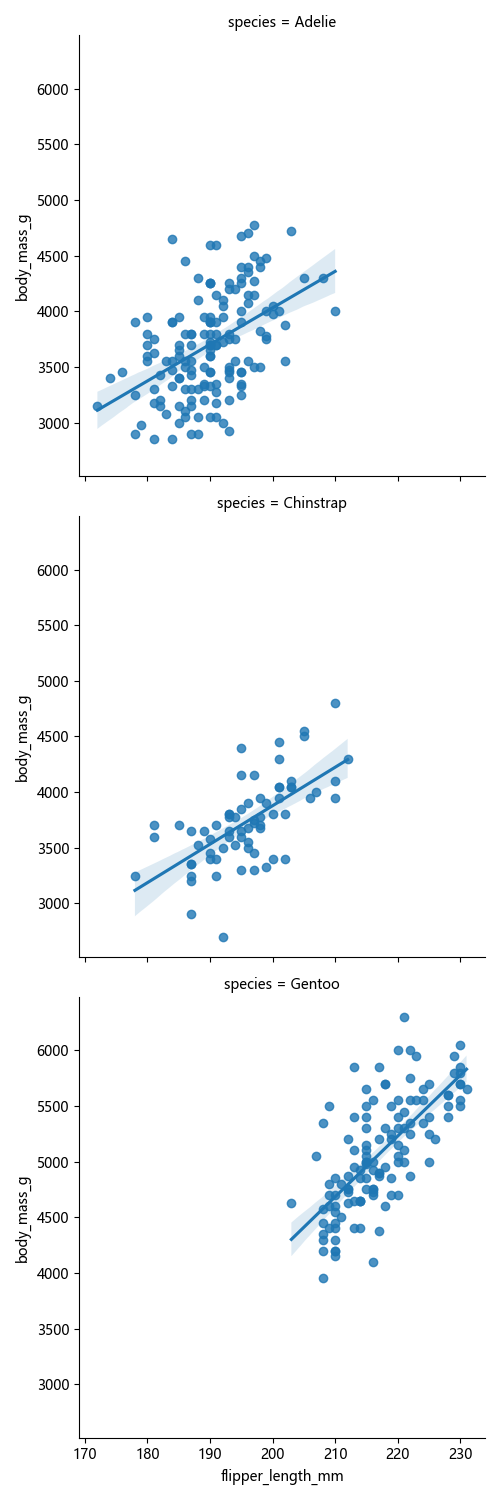
sns.lmplot(data=data, x="flipper_length_mm", y="body_mass_g", row="species")

plt.show()

📌 作用

• row="species" → 每个物种单独绘制回归图（纵向排列）。
  

---

4. 进阶用法

4.1 只显示回归线

sns.lmplot(data=data, x="flipper_length_mm", y="body_mass_g", hue="species", scatter=False)

plt.show()

📌 作用

• scatter=False → 只显示趋势线（适用于大数据集）。
  

---

4.2 多项式回归（order 参数）

sns.lmplot(data=data, x="flipper_length_mm", y="body_mass_g", order=2)

plt.show()

📌 作用

• order=2 进行二次回归拟合（曲线回归）。
  

---

4.3 关闭置信区间

sns.lmplot(data=data, x="flipper_length_mm", y="body_mass_g", ci=None)

plt.show()

📌 作用

• ci=None 取消置信区间。
  

---

5. sns.regplot() vs sns.lmplot()

	sns.regplot()	sns.lmplot()
hue 分类	❌ 不支持	✅ 支持
多子图	❌ 不支持	✅ col="var" / row="var"
适用场景	单个回归分析	分类别对比回归

---

6. 总结

✅ sns.lmplot() 适用于 多个类别的回归分析。
✅ 常见参数

• hue 按类别分色，col / row 生成多个子图。
• order=2 多项式回归，scatter=False 仅显示回归线。