


 这篇博客总结了skimage库的多个功能,包括曝光和颜色通道的调整、图像过滤与复原、对象分割、特征检测等。具体涉及免疫组织着色、边缘检测、多边形近似细分、DAISY特征描述、模板匹配、ORB和BRIEF二元描述符等技术。通过实例展示了skimage在图像处理中的应用。
skimage官网的示例。总结一下,作为以后研究的基础。
http://scikit-image.org/docs/stable/auto_examples/index.html#examples-gallery
使用曝光和颜色通道
如:免疫组织的分离着色、自适应的灰度滤波器到rgb图形、区域最大化滤波、局部直方图均衡、Gamma和log对比调节、直方图均衡、为灰度图着色
边缘和直线如:寻找轮廓、凸包、canny边缘检测、Marching Cubes、主动轮廓模型、边缘操作、画形状、画随机形状、直线的霍夫变换、近似细分的多边形、圆形和椭圆形的霍夫变换、骨架提取
如:密集daisy特征描述、原始梯度直方图、角点检测、模板匹配、补洞和寻找峰值、censure特征检测、multi-block local binary pattern for 纹理分类、Harr-like 特征检测、Blob检测、ORB特征检测和二元描述符、Brief二元描述符、Gabor/主要视觉cortex(simple cells)、GLCM纹理特征、形状索引、滑动窗口直方图、纹理分类的Gabor滤波器集合、局部二元模式 for 纹理分类
过滤器和复原
如:frangi 过滤器、hysteresis阈值、图像反卷积、均值过滤、图像反卷积2、图像修补、交叉熵、去噪、小波去噪、phase unwarpping、使用非局部均值滤波去噪—保留纹理
对象分割
如:基于RAGs的区域边界、正则化剪切、RAG阈值影响、采用紧凑的分水岭方法的规则分割、区域邻接图(RAG)、阈值、chan-vese分割、寻找局部最大化、niblack和sauvola阈值、标签图像区域、评估区域属性、随机游走的分割、分水岭分割、分水岭转换的标记、分割和超像素算法对比、寻找两个分割的交集、rag、rag合并、rags区域边界的分层合并、极值、形态学蛇形
几何转换和registration(不知道怎么翻译)如:漩涡(swirl)、生成图像金字塔、使用不同插值方式对于边缘的影响、rescale&resize&downscale、分段仿射变换、使用ransac方法的鲁棒三维线性模型评估、seam carving、基于ransac方法的鲁棒线性模型评估、结构的相似性索引、相位相关性分析、基本矩阵评估、radon转换、基于ransac的鲁棒匹配
其他的demo如:几何变换、形态学滤波、基于边缘和基于区域的分割对比、阈值转换、使用Haar-like的特征描述符用于面部分类、rank过滤
代码只贴了最核心的,原链接又完整的代码文件
1
是一种从3D体积中提取二维平面网格的算法。最早好像是应用在ct的重建上。大概就是对三维空间划分成为小立方体,然后判断对象对小立方体的占有情况:如果满就是内部,对于只占了立方体部分空间的对象表面,则通过切角的方法迭代逼近,也因此会形成很多三角网格。
(有道翻译)这可以被概念化为在地形或天气地图上的等值线的3D概括。它的工作原理是遍历整个卷,寻找那些跨越了兴趣级别的区域。如果发现了这些区域,就会生成三角测量并将其添加到输出网格中。最后的结果是一组顶点和一组三角形的面。

# Generate a level set about zero of two identical ellipsoids in 3D
ellip_base = ellipsoid(6, 10, 16, levelset=True)
ellip_double = np.concatenate((ellip_base[:-1, ...],
                               ellip_base[2:, ...]), axis=0)

# Use marching cubes to obtain the surface mesh of these ellipsoids
verts, faces, normals, values = measure.marching_cubes_lewiner(ellip_double, 0)
在图像1中对直线或边缘的线条或边缘进行调整。它的工作原理是将一部分由图像定义的能量最小化,部分由样条的形状决定:长度和平滑度。最小化是在形状能量中隐式地完成的在图像能量中
img = data.astronaut()
img = rgb2gray(img)

s = np.linspace(0, 2*np.pi, 400)
x = 220 + 100*np.cos(s)
y = 100 + 100*np.sin(s)
init = np.array([x, y]).T

snake = active_contour(gaussian(img, 3),init, alpha=0.015, beta=10, gamma=0.001)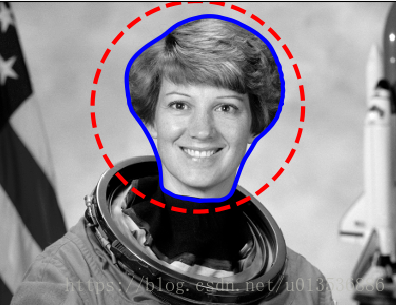
4Approximate and subdivide polygons
这个例子展示了如何近似(道格拉斯-peucker算法)和细分(b-splines)多边形链。
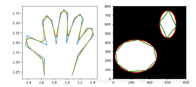
# subdivide polygon using 2nd degree B-Splines
new_hand = hand.copy()
for _ in range(5):
    new_hand = subdivide_polygon(new_hand, degree=2, preserve_ends=True)

# approximate subdivided polygon with Douglas-Peucker algorithm
appr_hand = approximate_polygon(new_hand, tolerance=0.02)
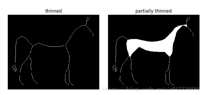
骨架化将二进制对象减少到1像素宽的表示。 这对于特征提取和/或表示对象的拓扑是很有用的。
- skeletonize :在每一次传递中,边界像素都被识别并删除,条件是它们不会破坏相应对象的连接性。
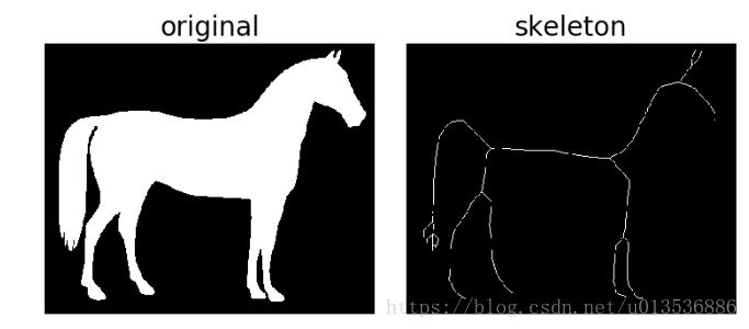
# Invert the horse image
image = invert(data.horse())

# perform skeletonization
skeleton = skeletonize(image)- skeletonize vs skeletonize 3d(略,原文有论文链接)
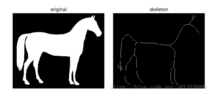
- Morphological thinning
skeleton = skeletonize(image)
thinned = thin(image)
thinned_partial = thin(image, max_iter=25)
菊花局部图像描述符是基于与筛选描述符相似的梯度方向直方图。它的形成方式是允许快速密集的提取,这对于例如具有特征的图像表示是很有用的。在本例中,为了便于说明,在很大的范围内提取了有限数量的菊花描述符。
img = data.camera()
descs, descs_img = daisy(img, step=180, radius=58, rings=2, histograms=6,
                         orientations=8, visualize=True)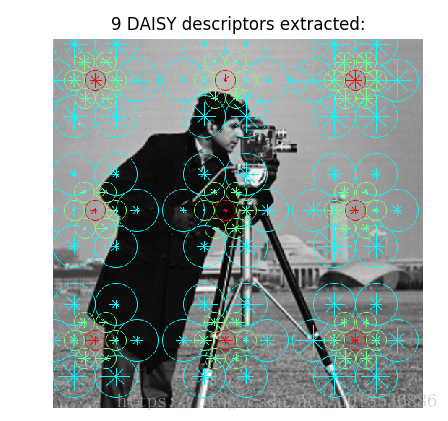
7Template Matching
我们使用模板匹配来识别图像补丁的出现(在本例中,一个以单个硬币为中心的子图像)。 在这里,我们返回一个匹配(完全相同的硬币),因此匹配模板结果中的最大值对应于硬币的位置。 其他的硬币看起来很相似,因此有局部最大值; 如果您期望多个匹配,您应该使用一个适当的峰值查找函数。 matchtemplate函数使用快速、规范化的交叉关联1来查找图像中模板的实例。 注意,匹配模板输出的峰值对应于模板的原点(即左上角)。image = data.coins()
coin = image[170:220, 75:130]
result = match_template(image, coin)
ij = np.unravel_index(np.argmax(result), result.shape)
x, y = ij[::-1]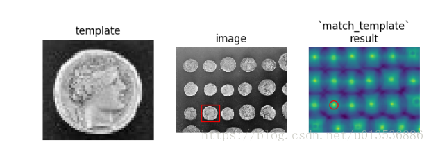
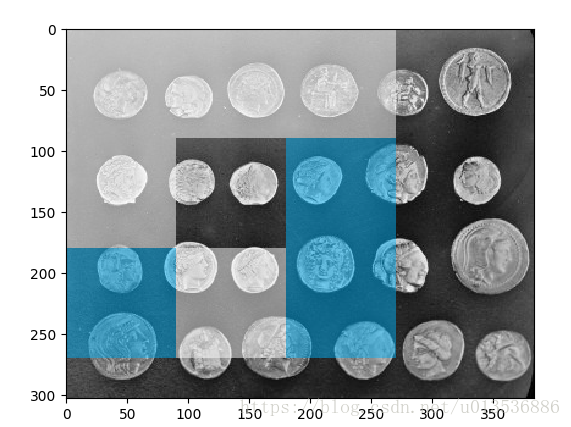
8 Multi-Block Local Binary Pattern for texture classification
这个例子展示了如何计算多块本地二进制模式(MB-LBP)特性以及如何将它们可视化。 这些特性的计算方法类似于本地二进制模式(LBPs),只是使用了求和块,而不是单个像素值。 MB-LBP是LBP的扩展,可以在恒定的时间内使用积分图像在多个尺度上计算。 9个同等大小的矩形用于计算一个特性。 对于每个矩形,计算出像素强度的总和。 将这些和中央矩形的比较结果与LBP相似(参见LBP)。 首先,我们生成一个图像来说明MB-LBP的功能:考虑一个(9、9)矩形,并将其划分为(3、3)块,然后我们应用MB-LBP。test_img = data.coins()
int_img = integral_image(test_img)
lbp_code = multiblock_lbp(int_img, 0, 0, 90, 90)
img = draw_multiblock_lbp(test_img, 0, 0, 90, 90,
lbp_code=lbp_code, alpha=0.5)
9 Haar-like feature descriptor
类似于haa的功能是简单的数字图像功能,这些特性是在实时的人脸检测器1中引入的。这些特性可以在恒定时间内以任何规模有效地计算,使用一个完整的图像1。在此之后,从这一大堆的潜在特性中选择了少量的关键特性(例如,使用AdaBoost学习算法,如1)。下面的例子将展示构建这个描述符族的机制。
images = [np.zeros((2, 2)), np.zeros((2, 2)),
          np.zeros((3, 3)), np.zeros((3, 3)),
          np.zeros((2, 2))]

feature_types = ['type-2-x', 'type-2-y',
                 'type-3-x', 'type-3-y',
                 'type-4']

fig, axs = plt.subplots(3, 2)
for ax, img, feat_t in zip(np.ravel(axs), images, feature_types):
    coord, _ = haar_like_feature_coord(img.shape[0], img.shape[1], feat_t)
    haar_feature = draw_haar_like_feature(img, 0, 0,
                                          img.shape[0],
                                          img.shape[1],
                                          coord,
                                          max_n_features=1,
                                          random_state=0)
    ax.imshow(haar_feature)
    ax.set_title(feat_t)
    ax.set_xticks([])
    ax.set_yticks([])

fig.suptitle('The different Haar-like feature descriptors')
plt.axis('off')
plt.show()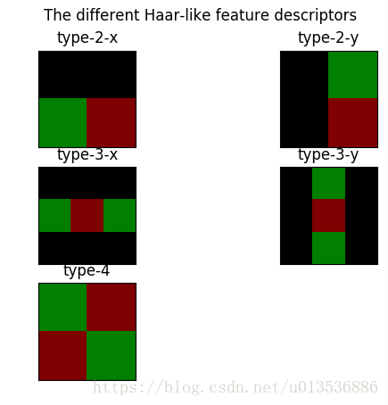
10 Blob Detection
- Laplacian of Gaussian (LoG)
- Difference of Gaussian (DoG)
- Determinant of Hessian (DoH
image = data.hubble_deep_field()[0:500, 0:500]
image_gray = rgb2gray(image)

blobs_log = blob_log(image_gray, max_sigma=30, num_sigma=10, threshold=.1)

# Compute radii in the 3rd column.
blobs_log[:, 2] = blobs_log[:, 2] * sqrt(2)

blobs_dog = blob_dog(image_gray, max_sigma=30, threshold=.1)
blobs_dog[:, 2] = blobs_dog[:, 2] * sqrt(2)

blobs_doh = blob_doh(image_gray, max_sigma=30, threshold=.01)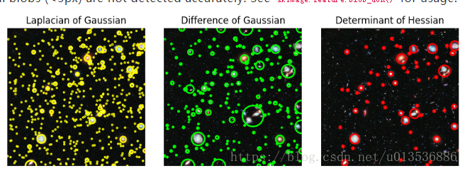
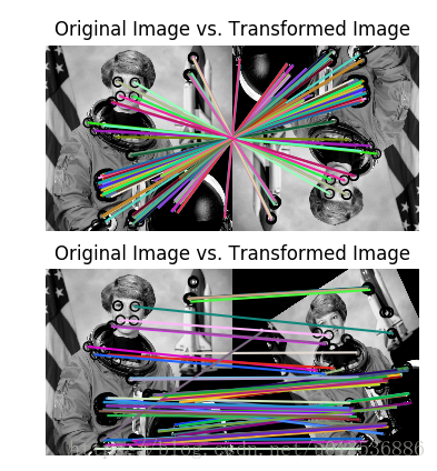
11 ORB feature detector and binary descriptor
这个例子演示了ORB特性检测和二进制描述算法。它使用了一种面向对象的快速检测方法和旋转的简要描述符。与简单的情况不同,ORB是相对尺度和旋转不变的,同时仍然使用非常有效的汉明距离度量来进行匹配。因此,它更适合于实时应用程序
img1 = rgb2gray(data.astronaut())
img2 = tf.rotate(img1, 180)
tform = tf.AffineTransform(scale=(1.3, 1.1), rotation=0.5,
                           translation=(0, -200))
img3 = tf.warp(img1, tform)

descriptor_extractor = ORB(n_keypoints=200)

descriptor_extractor.detect_and_extract(img1)
keypoints1 = descriptor_extractor.keypoints
descriptors1 = descriptor_extractor.descriptors

descriptor_extractor.detect_and_extract(img2)
keypoints2 = descriptor_extractor.keypoints
descriptors2 = descriptor_extractor.descriptors

descriptor_extractor.detect_and_extract(img3)
keypoints3 = descriptor_extractor.keypoints
descriptors3 = descriptor_extractor.descriptors

matches12 = match_descriptors(descriptors1, descriptors2, cross_check=True)
matches13 = match_descriptors(descriptors1, descriptors3, cross_check=True)

fig, ax = plt.subplots(nrows=2, ncols=1)

plt.gray()

plot_matches(ax[0], img1, img2, keypoints1, keypoints2, matches12)
ax[0].axis('off')
ax[0].set_title("Original Image vs. Transformed Image")

plot_matches(ax[1], img1, img3, keypoints1, keypoints3, matches13)
ax[1].axis('off')
ax[1].set_title("Original Image vs. Transformed Image")
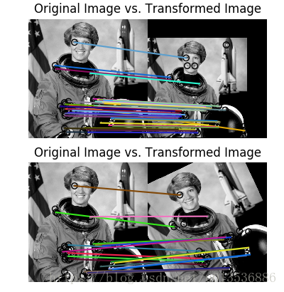
12 BRIEF binary descriptor
这个例子演示了简短的二进制描述算法。 描述符由相对较少的位组成,可以使用一组强度差测试来计算。 短的二进制描述符会导致低内存占用和基于汉明距离度量的非常有效的匹配。 简并不能提供旋转不变性。 通过在不同的尺度上检测和提取特征,可以实现尺度不变性。img1 = rgb2gray(data.astronaut())
tform = tf.AffineTransform(scale=(1.2, 1.2), translation=(0, -100))
img2 = tf.warp(img1, tform)
img3 = tf.rotate(img1, 25)
keypoints1 = corner_peaks(corner_harris(img1), min_distance=5)
keypoints2 = corner_peaks(corner_harris(img2), min_distance=5)
keypoints3 = corner_peaks(corner_harris(img3), min_distance=5)
extractor = BRIEF()
extractor.extract(img1, keypoints1)
keypoints1 = keypoints1[extractor.mask]
descriptors1 = extractor.descriptors
extractor.extract(img2, keypoints2)
keypoints2 = keypoints2[extractor.mask]
descriptors2 = extractor.descriptors
extractor.extract(img3, keypoints3)
keypoints3 = keypoints3[extractor.mask]
descriptors3 = extractor.descriptors
matches12 = match_descriptors(descriptors1, descriptors2, cross_check=True)
matches13 = match_descriptors(descriptors1, descriptors3, cross_check=True)
fig, ax = plt.subplots(nrows=2, ncols=1)
plt.gray()
plot_matches(ax[0], img1, img2, keypoints1, keypoints2, matches12)
ax[0].axis('off')
ax[0].set_title("Original Image vs. Transformed Image")
plot_matches(ax[1], img1, img3, keypoints1, keypoints3, matches13)
ax[1].axis('off')
ax[1].set_title("Original Image vs. Transformed Image")


 1559
1559

 被折叠的 条评论
为什么被折叠?
被折叠的 条评论
为什么被折叠?
 到【灌水乐园】发言


