Numpy quick fork

The Basics

NumPy’s main object is the homogeneous multidimensional array. It is a table of elements (usually numbers), all of the same type, indexed by a tuple of non-negative integers. In NumPy dimensions are called axes.

For example, the coordinates of a point in 3D space [1, 2, 1] has one axis. That axis has 3 elements in it, so we say it has a length of 3. In the example pictured below, the array has 2 axes. The first axis has a length of 2, the second axis has a length of 3.

[[ 1., 0., 0.],
[ 0., 1., 2.]]
NumPy’s array class is called ndarray. It is also known by the alias array. Note that numpy.array is not the same as the Standard Python Library class array.array, which only handles one-dimensional arrays and offers less functionality. The more important attributes of an ndarray object are:

ndarray.ndim
the number of axes (dimensions) of the array.
关于这个ndim 有点tricky ,参考：
https://www.zhihu.com/question/64894713

ndarray.shape
the dimensions of the array. This is a tuple of integers indicating the size of the array in each dimension. For a matrix with n rows and m columns, shape will be (n,m). The length of the shape tuple is therefore the number of axes, ndim.

ndarray.size
the total number of elements of the array. This is equal to the product of the elements of shape.

ndarray.dtype
an object describing the type of the elements in the array. One can create or specify dtype’s using standard Python types. Additionally NumPy provides types of its own. numpy.int32, numpy.int16, and numpy.float64 are some examples.

ndarray.itemsize
the size in bytes of each element of the array. For example, an array of elements of type float64 has itemsize 8 (=64/8), while one of type complex32 has itemsize 4 (=32/8). It is equivalent to ndarray.dtype.itemsize.

ndarray.data
the buffer containing the actual elements of the array. Normally, we won’t need to use this attribute because we will access the elements in an array using indexing facilities.

numpy.random.randint
refer to :
(https://numpy.org/doc/stable/reference/random/generated/numpy.random.randint.html#numpy.random.randint)

numpy.random.randint(low, high=None, size=None, dtype=int)
Return random integers from low (inclusive) to high (exclusive).
Return random integers from the “discrete uniform” distribution of the specified dtype in the “half-open” interval [low, high). If high is None (the default), then results are from [0, low).

0–50,需要显示指示size

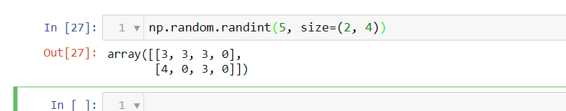
Generate a 2 x 4 array of ints between 0 and 4, inclusive:

NumPy 数据结构

>>> import numpy as np
>>> a = np.array([0, 0.5, 1.0, 1.5, 2.0])
>>> a
array([0. , 0.5, 1. , 1.5, 2. ])
>>> type(a)
<class 'numpy.ndarray'>

>>> a.sum()
5.0

>>> a.cumsum()  # running cumulative(累计） sum
array([0. , 0.5, 1.5, 3. , 5. ])
>>> 

另一个重要特征是ndarray 对象上定义的(向量化)数学运算:

>>> a*2
array([0., 1., 2., 3., 4.])
>>> a**2
array([0.  , 0.25, 1.  , 2.25, 4.  ])
>>> 

>>> np.sqrt(a)
array([0.        , 0.70710678, 1.        , 1.22474487, 1.41421356])

The function zeros creates an array full of zeros, the function ones creates an array full of ones, and the function empty creates an array whose initial content is random and depends on the state of the memory. By default, the dtype of the created array is float64.

>>> np.zeros((3, 5))
array([[0., 0., 0., 0., 0.],
       [0., 0., 0., 0., 0.],
       [0., 0., 0., 0., 0.]])

>>> np.ones(( 2,3), dtype=np.int16 )
array([[1, 1, 1],
       [1, 1, 1]], dtype=int16)
>>> 

https://numpy.org/doc/stable/user/quickstart.html

>>> np.empty( (2,3) )                                 # uninitialized
array([[1.39069238e-309, 1.39069238e-309, 1.39069238e-309],
       [1.39069238e-309, 1.39069238e-309, 1.39069238e-309]])
>>> 

To create sequences of numbers, NumPy provides the arange function which is analogous to the Python built-in range, but returns an array.

>>> np.arange( 10, 30, 5 )
array([10, 15, 20, 25])

>>> np.arange( 0, 2, 0.3 )                 # it accepts float arguments
array([0. , 0.3, 0.6, 0.9, 1.2, 1.5, 1.8])
>>> 

reshape

>>> b = np.arange(12).reshape(4,3)
>>> 
>>> b
array([[ 0,  1,  2],
       [ 3,  4,  5],
       [ 6,  7,  8],
       [ 9, 10, 11]])
>>> 

>>> print(np.arange(10000))
[   0    1    2 ... 9997 9998 9999]
>>>
>

If an array is too large to be printed, NumPy automatically skips the central part of the array and only prints the corners:

>>>
>>> print(np.arange(10000))
[   0    1    2 ... 9997 9998 9999]
>>>
>>> print(np.arange(10000).reshape(100,100))
[[   0    1    2 ...   97   98   99]
 [ 100  101  102 ...  197  198  199]
 [ 200  201  202 ...  297  298  299]
 ...
 [9700 9701 9702 ... 9797 9798 9799]
 [9800 9801 9802 ... 9897 9898 9899]
 [9900 9901 9902 ... 9997 9998 9999]]

To disable this behaviour and force NumPy to print the entire array, you can change the printing options using set_printoptions.

>>
>>> np.set_printoptions(threshold=sys.maxsize)       # sys module should be imported

>>> a = np.array( [20,30,40,50] )
>>> b = np.arange( 4 )
>>> b
array([0, 1, 2, 3])
>>> c = a-b
>>> c
array([20, 29, 38, 47])
>>> b**2
array([0, 1, 4, 9])
>>> 10*np.sin(a)
array([ 9.12945251, -9.88031624,  7.4511316 , -2.62374854])
>>> a<35
array([ True,  True, False, False])

矩阵的点乘和矩阵乘

Unlike in many matrix languages, the product operator * operates elementwise in NumPy arrays. The matrix product can be performed using the @ operator (in python >=3.5) or the dot function or method:

>>>
>>> A = np.array( [[1,1],
...                [0,1]] )
>>> B = np.array( [[2,0],
...                [3,4]] )
>>> A * B                       # elementwise product  点乘 
array([[2, 0],
       [0, 4]])
>>> A @ B                       # matrix product矩阵乘法
array([[5, 4],
       [3, 4]])
>>> A.dot(B)                    # another matrix product矩阵乘法
array([[5, 4],
       [3, 4]])

点乘,也就是每行乘以每行：

by specifying the axis parameter you can apply an operation along the specified axis of an array:

>>>
>>> b = np.arange(12).reshape(3,4)
>>> b
array([[ 0,  1,  2,  3],
       [ 4,  5,  6,  7],
       [ 8,  9, 10, 11]])
>>>
>>> b.sum(axis=0)                            # sum of each column
array([12, 15, 18, 21])
>>>
>>> b.min(axis=1)                            # min of each row
array([0, 4, 8])
>>>
>>> b.cumsum(axis=1)                         # cumulative sum along each row
array([[ 0,  1,  3,  6],
       [ 4,  9, 15, 22],
       [ 8, 17, 27, 38]])

axis =0 就是按列累加

>>> b.cumsum(axis =0)
array([[ 0,  1,  2,  3],
       [ 4,  6,  8, 10],
       [12, 15, 18, 21]], dtype=int32)

linspace
numpy.linspace(start, stop, num=50, endpoint=True, retstep=False, dtype=None)

在指定的间隔内返回均匀间隔的数字。

返回num均匀分布的样本，在[start, stop]。

这个区间的端点可以任意的被排除在外,方法是通过设置参数：
endpoint : bool, optional

如果是真，则一定包括stop，如果为False，一定不会有stop

>>> np.linspace(1, 10, 10)
array([ 1.,  2.,  3.,  4.,  5.,  6.,  7.,  8.,  9., 10.])
>>> np.linspace(1, 100, 100)
array([  1.,   2.,   3.,   4.,   5.,   6.,   7.,   8.,   9.,  10.,  11.,
        12.,  13.,  14.,  15.,  16.,  17.,  18.,  19.,  20.,  21.,  22.,
        23.,  24.,  25.,  26.,  27.,  28.,  29.,  30.,  31.,  32.,  33.,
        34.,  35.,  36.,  37.,  38.,  39.,  40.,  41.,  42.,  43.,  44.,
        45.,  46.,  47.,  48.,  49.,  50.,  51.,  52.,  53.,  54.,  55.,
        56.,  57.,  58.,  59.,  60.,  61.,  62.,  63.,  64.,  65.,  66.,
        67.,  68.,  69.,  70.,  71.,  72.,  73.,  74.,  75.,  76.,  77.,
        78.,  79.,  80.,  81.,  82.,  83.,  84.,  85.,  86.,  87.,  88.,
        89.,  90.,  91.,  92.,  93.,  94.,  95.,  96.,  97.,  98.,  99.,
       100.])
>>> 

>>> from numpy import pi
>>> np.linspace( 0, 2, 9 )                 # 9 numbers from 0 to 2
array([0.  , 0.25, 0.5 , 0.75, 1.  , 1.25, 1.5 , 1.75, 2.  ])
>>> x = np.linspace( 0, 2*pi, 100 )        # useful to evaluate function at lots of points
>>> f = np.sin(x)