


DNN前向传播算法和反向传播算法
感知机的模型大家都比较熟悉,它是一个有若干输入和一个输出的模型,如下图:
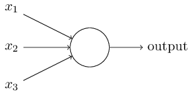
输出和输入之间学习到一个线性关系,得到中间输出结果:
接着是一个神经元激活函数: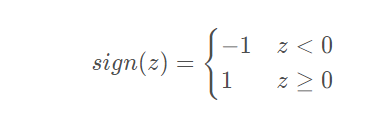
从而得到我们想要的输出结果1或者-1。
这个模型只能用于二元分类,且无法学习比较复杂的非线性模型,因此在工业界无法使用。
而神经网络则在感知机的模型上做了扩展,总结下主要有三点:
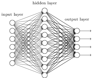
1)加入了隐藏层,隐藏层可以有多层,增强模型的表达能力,如下图实例,当然增加了这么多隐藏层模型的复杂度也增加了好多。
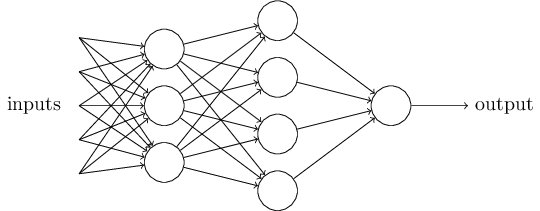
2)输出层的神经元也可以不止一个输出,可以有多个输出,这样模型可以灵活的应用于分类回归,以及其他的机器学习领域比如降维和聚类等。多个神经元输出的输出层对应的一个实例如下图,输出层现在有4个神经元了。
3) 对激活函数做扩展,感知机的激活函数是sign(z),虽然简单但是处理能力有限,因此神经网络中一般使用的其他的激活函数,比如我们在逻辑回归里面使用过的Sigmoid函数,即: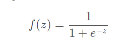
DNN有时也叫做多层感知机(Multi-Layer perceptron,MLP), 名字实在是多。后面我们讲到的神经网络都默认为DNN。
还有后来出现的tanx, softmax,和ReLU等。通过使用不同的激活函数,神经网络的表达能力进一步增强。对于各种常用的激活函数,我随后会整理一份资料。
DNN损失函数和激活函数的选择
1)均方误差损失+sigmoid激活,梯度变化小,收敛速度慢,难以找到最优解。
2)使用交叉熵损失函数+Sigmoid激活函数改进DNN算法收敛速度,容易梯度消失。
3) 使用对数似然损失函数和softmax激活函数进行DNN分类输出
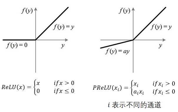
4) ReLU激活函数解决梯度消失。
5) tanh:这个是sigmoid的变种
6) softplus:这个其实就是sigmoid函数的原函数
7)PReLU:从名字就可以看出它是ReLU的变种,特点是如果未激活值小于0,不是简单粗暴的直接变为0,而是进行一定幅度的缩小。如下图。当然,由于ReLU的成功,有很多的跟风者,有其他各种变种ReLU,这里就不多提了。
1)如果使用sigmoid激活函数,则交叉熵损失函数一般肯定比均方差损失函数好。
2)如果是DNN用于分类,则一般在输出层使用softmax激活函数和对数似然损失函数。
3)ReLU激活函数对梯度消失问题有一定程度的解决,尤其是在CNN模型中。
Boltzmann Machines
Boltzmann machines were invented in 1985 by Geoffrey Hinton and Terrence Sejnow‐ ski. Just like Hopfield nets, they are fully connected ANNs, but they are based on sto‐chastic neurons: instead of using a deterministic step function to decide what value to output, these neurons output 1 with some probability, and 0 otherwise. The probabil‐ ity function that these ANNs use is based on the Boltzmann distribution (used in statistical mechanics) hence their name. Equation E-1 gives the probability that a par‐ ticular neuron will output a 1. Equation E-1. Probability that the ith neuron will output 1


Neurons in Boltzmann machines are separated into two groups: visible units and hid‐ den units (see Figure E-2). All neurons work in the same stochastic way, but the visi‐ ble units are the ones that receive the inputs and from which outputs are read.

玻尔兹曼机:Markov RandomFiled with hidden nodes(隐马尔科夫随机场)
Because of its stochastic nature, a Boltzmann machine will never stabilize into a fixed configuration, but instead it will keep switching between many configurations. If it is left running for a sufficiently long time, the probability of observing a particular con‐ figuration will only be a function of the connection weights and bias terms, not of the original configuration (similarly, after you shuffle a deck of cards for long enough, the configuration of the deck does not depend on the initial state). When the network reaches this state where the original configuration is “forgotten,” it is said to be in thermal equilibrium (although its configuration keeps changing all the time). By set‐ ting the network parameters appropriately, letting the network reach thermal equili‐ brium, and then observing its state, we can simulate a wide range of probability distributions. This is called a generative model.
Training a Boltzmann machine means finding the parameters that will make the net‐ work approximate the training set’s probability distribution. For example, if there are three visible neurons and the training set contains 75% (0, 1, 1) triplets, 10% (0, 0, 1) triplets, and 15% (1, 1, 1) triplets, then after training a Boltzmann machine, you could use it to generate random binary triplets with about the same probability distribu‐ tion. For example, about 75% of the time it would output the (0, 1, 1) triplet. Such a generative model can be used in a variety of ways. For example, if it is trained on images, and you provide an incomplete or noisy image to the network, it will automatically “repair” the image in a reasonable way. You can also use a generative model for classification. Just add a few visible neurons to encode the training image’s class (e.g., add 10 visible neurons and turn on only the fifth neuron when the training image represents a 5). Then, when given a new image, the network will automatically turn on the appropriate visible neurons, indicating the image’s class (e.g., it will turn on the fifth visible neuron if the image represents a 5). Unfortunately, there is no efficient technique to train Boltzmann machines. However, fairly efficient algorithms have been developed to train restricted Boltzmann machines (RBM).
Restricted Boltzmann Machines
受限玻尔兹曼机本身是一个基于二分图的无向图的模型,图中的一部分是可见层,一部分是隐藏层,并且同层之间的单元和单元之间没有任何连接。

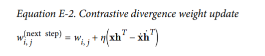
A very efficient training algorithm, called Contrastive Divergence, was introduced in 2005 by Miguel Á. Carreira-Perpiñán and Geoffrey Hinton. 1 Here is how it works: for each training instance x, the algorithm starts by feeding it to the network by setting the state of the visible units to x1 , x2 , ⋯, xn . Then you compute the state of the hidden units by applying the stochastic equation described before (Equation E-1). This gives you a hidden vector h (where hi is equal to the state of the ith unit). Next you compute the state of the visible units, by applying the same stochastic equation. This gives you a vector ᅴ˙. Then once again you compute the state of the hidden units, which gives you a vector ᅤ ˙ .
The great benefit of this algorithm it that it does not require waiting for the network to reach thermal equilibrium: it just goes forward, backward, and forward again, and that’s it. This makes it incomparably more efficient than previous algorithms, and it was a key ingredient to the first success of Deep Learning based on multiple stacked RBMs.
Deep Belief Nets(DBN)
Several layers of RBMs can be stacked; the hidden units of the first-level RBM serves as the visible units for the second-layer RBM, and so on. Such an RBM stack is called a deep belief net (DBN).
Yee-Whye Teh, one of Geoffrey Hinton’s students, observed that it was possible to train DBNs one layer at a time using Contrastive Divergence, starting with the lowerlayers and then gradually moving up to the top layers. This led to the groundbreaking article that kickstarted the Deep Learning tsunami in 2006. 2
Just like RBMs, DBNs learn to reproduce the probability distribution of their inputs, without any supervision. However, they are much better at it, for the same reason that deep neural networks are more powerful than shallow ones: real-world data is often organized in hierarchical patterns, and DBNs take advantage of that. Their lower lay‐ ers learn low-level features in the input data, while higher layers learn high-level fea‐ tures. Just like RBMs, DBNs are fundamentally unsupervised, but you can also train them in a supervised manner by adding some visible units to represent the labels. More‐ over, one great feature of DBNs is that they can be trained in a semisupervised fash‐ ion. Figure E-4 represents such a DBN configured for semisupervised learning.

First, the RBM 1 is trained without supervision. It learns low-level features in the training data. Then RBM 2 is trained with RBM 1’s hidden units as inputs, again without supervision: it learns higher-level features (note that RBM 2’s hidden units include only the three rightmost units, not the label units). Several more RBMs could be stacked this way, but you get the idea. So far, training was 100% unsupervised.
Lastly, RBM 3 is trained using both RBM 2’s hidden units as inputs, as well as extra visible units used to represent the target labels (e.g., a one-hot vector representing the instance class). It learns to associate high-level features with training labels. This is the supervised step.
At the end of training, if you feed RBM 1 a new instance, the signal will propagate up to RBM 2, then up to the top of RBM 3, and then back down to the label units; hope‐ fully, the appropriate label will light up. This is how a DBN can be used for classifica‐ tion.
One great benefit of this semisupervised approach is that you don’t need much labeled training data. If the unsupervised RBMs do a good enough job, then only a small amount of labeled training instances per class will be necessary. Similarly, a baby learns to recognize objects without supervision, so when you point to a chair and say “chair,” the baby can associate the word “chair” with the class of objects it has already learned to recognize on its own. You don’t need to point to every single chair and say “chair”; only a few examples will suffice (just enough so the baby can be sure that you are indeed referring to the chair, not to its color or one of the chair’s parts).
One great benefit of this semisupervised approach is that you don’t need much labeled training data. If the unsupervised RBMs do a good enough job, then only a small amount of labeled training instances per class will be necessary. Similarly, a baby learns to recognize objects without supervision, so when you point to a chair and say “chair,” the baby can associate the word “chair” with the class of objects it has already learned to recognize on its own. You don’t need to point to every single chair and say “chair”; only a few examples will suffice (just enough so the baby can be sure that you are indeed referring to the chair, not to its color or one of the chair’s parts). Quite amazingly, DBNs can also work in reverse. If you activate one of the label units, the signal will propagate up to the hidden units of RBM 3, then down to RBM 2, and then RBM 1, and a new instance will be output by the visible units of RBM 1. This new instance will usually look like a regular instance of the class whose label unit you activated. This generative capability of DBNs is quite powerful. For example, it has been used to automatically generate captions for images, and vice versa: first a DBN is trained (without supervision) to learn features in images, and another DBN is trained (again without supervision) to learn features in sets of captions (e.g., “car” often comes with “automobile”). Then an RBM is stacked on top of both DBNs and trained with a set of images along with their captions; it learns to associate high-level features in images with high-level features in captions. Next, if you feed the image DBN an image of a car, the signal will propagate through the network, up to the top-level RBM, and back down to the bottom of the caption DBN, producing a caption. Due to the stochastic nature of RBMs and DBNs, the caption will keep changing randomly, but it will generally be appropriate for the image. If you generate a few hundred cap‐ tions, the most frequently generated ones will likely be a good description of the image.3
https://blog.csdn.net/zhanglu_wind/article/details/78949020
Deep Belief Networks
Note
This section assumes the reader has already read through Classifying MNIST digits using Logistic Regression and Multilayer Perceptron and Restricted Boltzmann Machines (RBM). Additionally it uses the following Theano functions and concepts: T.tanh, shared variables, basic arithmetic ops, T.grad, Random numbers, floatX. If you intend to run the code on GPU also read GPU.
Note
The code for this section is available for download here.
Deep Belief Networks
[Hinton06] showed that RBMs can be stacked and trained in a greedy manner to form so-called Deep Belief Networks (DBN). DBNs are graphical models which learn to extract a deep hierarchical representation of the training data. They model the joint distribution between observed vector  and the
  hidden layers
  as follows:
(1)
where  ,
,  is a conditional distribution for the visible units conditioned on the hidden units of the RBM at level
  , and
, and  is the visible-hidden joint distribution in the top-level RBM. This is illustrated in the figure below.

The principle of greedy layer-wise unsupervised training can be applied to DBNs with RBMs as the building blocks for each layer [Hinton06], [Bengio07]. The process is as follows:
1. Train the first layer as an RBM that models the raw input  as its visible layer.
2. Use that first layer to obtain a representation of the input that will be used as data for the second layer. Two common solutions exist. This representation can be chosen as being the mean activations  or samples of
  .
.
3. Train the second layer as an RBM, taking the transformed data (samples or mean activations) as training examples (for the visible layer of that RBM).
4. Iterate (2 and 3) for the desired number of layers, each time propagating upward either samples or mean values.
5. Fine-tune all the parameters of this deep architecture with respect to a proxy for the DBN log- likelihood, or with respect to a supervised training criterion (after adding extra learning machinery to convert the learned representation into supervised predictions, e.g. a linear classifier).
In this tutorial, we focus on fine-tuning via supervised gradient descent. Specifically, we use a logistic regression classifier to classify the input based on the output of the last hidden layer  of the DBN. Fine-tuning is then performed via supervised gradient descent of the negative log-likelihood cost function. Since the supervised gradient is only non-null for the weights and hidden layer biases of each layer (i.e. null for the visible biases of each RBM), this procedure is equivalent to initializing the parameters of a deep MLP with the weights and hidden layer biases obtained with the unsupervised training strategy.
Justifying Greedy-Layer Wise Pre-Training
Why does such an algorithm work ? Taking as example a 2-layer DBN with hidden layers  and
and  (with respective weight parameters
  and
and  ), [Hinton06] established (see also Bengio09]_ for a detailed derivation) that
  can be rewritten as,
(2)
 represents the KL divergence between the posterior
  of the first RBM if it were standalone, and the probability
  for the same layer but defined by the entire DBN (i.e. taking into account the prior
  defined by the top-level RBM).
  is the entropy of the distribution .
It can be shown that if we initialize both hidden layers such that  ,
,  and the KL divergence term is null. If we learn the first level RBM and then keep its parameters fixed, optimizing Eq. (2) with respect to can thus only increase the likelihood
  .
.
Also, notice that if we isolate the terms which depend only on , we get:

Optimizing this with respect to amounts to training a second-stage RBM, using the output of as the training distribution, when is sampled from the training distribution for the first RBM.
Implementation
To implement DBNs in Theano, we will use the class defined in the Restricted Boltzmann Machines (RBM) tutorial. One can also observe that the code for the DBN is very similar with the one for SdA, because both involve the principle of unsupervised layer-wise pre-training followed by supervised fine-tuning as a deep MLP. The main difference is that we use the RBM class instead of the dA class.
We start off by defining the DBN class which will store the layers of the MLP, along with their associated RBMs. Since we take the viewpoint of using the RBMs to initialize an MLP, the code will reflect this by seperating as much as possible the RBMs used to initialize the network and the MLP used for classification.
class DBN(object):
    """Deep Belief Network

    A deep belief network is obtained by stacking several RBMs on top of each
    other. The hidden layer of the RBM at layer `i` becomes the input of the
    RBM at layer `i+1`. The first layer RBM gets as input the input of the
    network, and the hidden layer of the last RBM represents the output. When
    used for classification, the DBN is treated as a MLP, by adding a logistic
    regression layer on top.
    """

    def __init__(self, numpy_rng, theano_rng=None, n_ins=784,
                 hidden_layers_sizes=[500, 500], n_outs=10):
        """This class is made to support a variable number of layers.

        :type numpy_rng: numpy.random.RandomState
        :param numpy_rng: numpy random number generator used to draw initial
                    weights

        :type theano_rng: theano.tensor.shared_randomstreams.RandomStreams
        :param theano_rng: Theano random generator; if None is given one is
                           generated based on a seed drawn from `rng`

        :type n_ins: int
        :param n_ins: dimension of the input to the DBN

        :type hidden_layers_sizes: list of ints
        :param hidden_layers_sizes: intermediate layers size, must contain
                               at least one value

        :type n_outs: int
        :param n_outs: dimension of the output of the network
        """

        self.sigmoid_layers = []
        self.rbm_layers = []
        self.params = []
        self.n_layers = len(hidden_layers_sizes)

        assert self.n_layers > 0

        if not theano_rng:
            theano_rng = MRG_RandomStreams(numpy_rng.randint(2 ** 30))

        # allocate symbolic variables for the data

        # the data is presented as rasterized images
        self.x = T.matrix('x')

        # the labels are presented as 1D vector of [int] labels
        self.y = T.ivector('y')
self.sigmoid_layers will store the feed-forward graphs which together form the MLP, while self.rbm_layers will store the RBMs used to pretrain each layer of the MLP.
Next step, we construct n_layers sigmoid layers (we use the HiddenLayer class introduced in Multilayer Perceptron, with the only modification that we replaced the non-linearity from tanh to the logistic function  ) and
) and n_layers RBMs, where n_layers is the depth of our model. We link the sigmoid layers such that they form an MLP, and construct each RBM such that they share the weight matrix and the hidden bias with its corresponding sigmoid layer.
        for i in range(self.n_layers):
            # construct the sigmoidal layer

            # the size of the input is either the number of hidden
            # units of the layer below or the input size if we are on
            # the first layer
            if i == 0:
                input_size = n_ins
            else:
                input_size = hidden_layers_sizes[i - 1]

            # the input to this layer is either the activation of the
            # hidden layer below or the input of the DBN if you are on
            # the first layer
            if i == 0:
                layer_input = self.x
            else:
                layer_input = self.sigmoid_layers[-1].output

            sigmoid_layer = HiddenLayer(rng=numpy_rng,
                                        input=layer_input,
                                        n_in=input_size,
                                        n_out=hidden_layers_sizes[i],
                                        activation=T.nnet.sigmoid)

            # add the layer to our list of layers
            self.sigmoid_layers.append(sigmoid_layer)

            # its arguably a philosophical question...  but we are
            # going to only declare that the parameters of the
            # sigmoid_layers are parameters of the DBN. The visible
            # biases in the RBM are parameters of those RBMs, but not
            # of the DBN.
            self.params.extend(sigmoid_layer.params)

            # Construct an RBM that shared weights with this layer
            rbm_layer = RBM(numpy_rng=numpy_rng,
                            theano_rng=theano_rng,
                            input=layer_input,
                            n_visible=input_size,
                            n_hidden=hidden_layers_sizes[i],
                            W=sigmoid_layer.W,
                            hbias=sigmoid_layer.b)
            self.rbm_layers.append(rbm_layer)
All that is left is to stack one last logistic regression layer in order to form an MLP. We will use the LogisticRegression class introduced in Classifying MNIST digits using Logistic Regression.
        self.logLayer = LogisticRegression(
            input=self.sigmoid_layers[-1].output,
            n_in=hidden_layers_sizes[-1],
            n_out=n_outs)
        self.params.extend(self.logLayer.params)

        # compute the cost for second phase of training, defined as the
        # negative log likelihood of the logistic regression (output) layer
        self.finetune_cost = self.logLayer.negative_log_likelihood(self.y)

        # compute the gradients with respect to the model parameters
        # symbolic variable that points to the number of errors made on the
        # minibatch given by self.x and self.y
        self.errors = self.logLayer.errors(self.y)
The class also provides a method which generates training functions for each of the RBMs. They are returned as a list, where element  is a function which implements one step of training for the
 RBM at layer .
    def pretraining_functions(self, train_set_x, batch_size, k):
        '''Generates a list of functions, for performing one step of
        gradient descent at a given layer. The function will require
        as input the minibatch index, and to train an RBM you just
        need to iterate, calling the corresponding function on all
        minibatch indexes.

        :type train_set_x: theano.tensor.TensorType
        :param train_set_x: Shared var. that contains all datapoints used
                            for training the RBM
        :type batch_size: int
        :param batch_size: size of a [mini]batch
        :param k: number of Gibbs steps to do in CD-k / PCD-k

        '''

        # index to a [mini]batch
        index = T.lscalar('index')  # index to a minibatch
In order to be able to change the learning rate during training, we associate a Theano variable to it that has a default value.
        learning_rate = T.scalar('lr')  # learning rate to use

        # begining of a batch, given `index`
        batch_begin = index * batch_size
        # ending of a batch given `index`
        batch_end = batch_begin + batch_size

        pretrain_fns = []
        for rbm in self.rbm_layers:

            # get the cost and the updates list
            # using CD-k here (persisent=None) for training each RBM.
            # TODO: change cost function to reconstruction error
            cost, updates = rbm.get_cost_updates(learning_rate,
                                                 persistent=None, k=k)

            # compile the theano function
            fn = theano.function(
                inputs=[index, theano.In(learning_rate, value=0.1)],
                outputs=cost,
                updates=updates,
                givens={
                    self.x: train_set_x[batch_begin:batch_end]
                }
            )
            # append `fn` to the list of functions
            pretrain_fns.append(fn)

        return pretrain_fns
Now any function pretrain_fns[i] takes as arguments index and optionally lr – the learning rate. Note that the names of the parameters are the names given to the Theano variables (e.g. lr) when they are constructed and not the name of the python variables (e.g. learning_rate). Keep this in mind when working with Theano. Optionally, if you provide k (the number of Gibbs steps to perform in CD or PCD) this will also become an argument of your function.
In the same fashion, the DBN class includes a method for building the functions required for finetuning ( a train_model, a validate_model and a test_model function).
    def build_finetune_functions(self, datasets, batch_size, learning_rate):
        '''Generates a function `train` that implements one step of
        finetuning, a function `validate` that computes the error on a
        batch from the validation set, and a function `test` that
        computes the error on a batch from the testing set

        :type datasets: list of pairs of theano.tensor.TensorType
        :param datasets: It is a list that contain all the datasets;
                        the has to contain three pairs, `train`,
                        `valid`, `test` in this order, where each pair
                        is formed of two Theano variables, one for the
                        datapoints, the other for the labels
        :type batch_size: int
        :param batch_size: size of a minibatch
        :type learning_rate: float
        :param learning_rate: learning rate used during finetune stage

        '''

        (train_set_x, train_set_y) = datasets[0]
        (valid_set_x, valid_set_y) = datasets[1]
        (test_set_x, test_set_y) = datasets[2]

        # compute number of minibatches for training, validation and testing
        n_valid_batches = valid_set_x.get_value(borrow=True).shape[0]
        n_valid_batches //= batch_size
        n_test_batches = test_set_x.get_value(borrow=True).shape[0]
        n_test_batches //= batch_size

        index = T.lscalar('index')  # index to a [mini]batch

        # compute the gradients with respect to the model parameters
        gparams = T.grad(self.finetune_cost, self.params)

        # compute list of fine-tuning updates
        updates = []
        for param, gparam in zip(self.params, gparams):
            updates.append((param, param - gparam * learning_rate))

        train_fn = theano.function(
            inputs=[index],
            outputs=self.finetune_cost,
            updates=updates,
            givens={
                self.x: train_set_x[
                    index * batch_size: (index + 1) * batch_size
                ],
                self.y: train_set_y[
                    index * batch_size: (index + 1) * batch_size
                ]
            }
        )

        test_score_i = theano.function(
            [index],
            self.errors,
            givens={
                self.x: test_set_x[
                    index * batch_size: (index + 1) * batch_size
                ],
                self.y: test_set_y[
                    index * batch_size: (index + 1) * batch_size
                ]
            }
        )

        valid_score_i = theano.function(
            [index],
            self.errors,
            givens={
                self.x: valid_set_x[
                    index * batch_size: (index + 1) * batch_size
                ],
                self.y: valid_set_y[
                    index * batch_size: (index + 1) * batch_size
                ]
            }
        )

        # Create a function that scans the entire validation set
        def valid_score():
            return [valid_score_i(i) for i in range(n_valid_batches)]

        # Create a function that scans the entire test set
        def test_score():
            return [test_score_i(i) for i in range(n_test_batches)]

        return train_fn, valid_score, test_score
Note that the returned valid_score and test_score are not Theano functions, but rather Python functions. These loop over the entire validation set and the entire test set to produce a list of the losses obtained over these sets.
Putting it all together
The few lines of code below constructs the deep belief network:
    numpy_rng = numpy.random.RandomState(123)
    print('... building the model')
    # construct the Deep Belief Network
    dbn = DBN(numpy_rng=numpy_rng, n_ins=28 * 28,
              hidden_layers_sizes=[1000, 1000, 1000],
              n_outs=10)
There are two stages in training this network: (1) a layer-wise pre-training and (2) a fine-tuning stage.
For the pre-training stage, we loop over all the layers of the network. For each layer, we use the compiled theano function which determines the input to the i-th level RBM and performs one step of CD-k within this RBM. This function is applied to the training set for a fixed number of epochs given by pretraining_epochs.
    #########################
    # PRETRAINING THE MODEL #
    #########################
    print('... getting the pretraining functions')
    pretraining_fns = dbn.pretraining_functions(train_set_x=train_set_x,
                                                batch_size=batch_size,
                                                k=k)

    print('... pre-training the model')
    start_time = timeit.default_timer()
    # Pre-train layer-wise
    for i in range(dbn.n_layers):
        # go through pretraining epochs
        for epoch in range(pretraining_epochs):
            # go through the training set
            c = []
            for batch_index in range(n_train_batches):
                c.append(pretraining_fns[i](index=batch_index,
                                            lr=pretrain_lr))
            print('Pre-training layer %i, epoch %d, cost ' % (i, epoch), end=' ')
            print(numpy.mean(c, dtype='float64'))

    end_time = timeit.default_timer()
The fine-tuning loop is very similar to the one in the Multilayer Perceptron tutorial, the only difference being that we now use the functions given by build_finetune_functions.
Running the Code
The user can run the code by calling:
python code/DBN.py
With the default parameters, the code runs for 100 pre-training epochs with mini-batches of size 10. This corresponds to performing 500,000 unsupervised parameter updates. We use an unsupervised learning rate of 0.01, with a supervised learning rate of 0.1. The DBN itself consists of three hidden layers with 1000 units per layer. With early-stopping, this configuration achieved a minimal validation error of 1.27 with corresponding test error of 1.34 after 46 supervised epochs.
On an Intel(R) Xeon(R) CPU X5560 running at 2.80GHz, using a multi-threaded MKL library (running on 4 cores), pretraining took 615 minutes with an average of 2.05 mins/(layer * epoch). Fine-tuning took only 101 minutes or approximately 2.20 mins/epoch.
Hyper-parameters were selected by optimizing on the validation error. We tested unsupervised learning rates in  and supervised learning rates in
  . We did not use any form of regularization besides early-stopping, nor did we optimize over the number of pretraining updates.
Tips and Tricks
One way to improve the running time of your code (given that you have sufficient memory available), is to compute the representation of the entire dataset at layer i in a single pass, once the weights of the  -th layers have been fixed. Namely, start by training your first layer RBM. Once it is trained, you can compute the hidden units values for every example in the dataset and store this as a new dataset which is used to train the 2nd layer RBM. Once you trained the RBM for layer 2, you compute, in a similar fashion, the dataset for layer 3 and so on. This avoids calculating the intermediate (hidden layer) representations,
 pretraining_epochs times at the expense of increased memory usage.


 1万+
1万+


 被折叠的 条评论
为什么被折叠?
被折叠的 条评论
为什么被折叠?
 到【灌水乐园】发言


