统计推断week4

4.1 P值

P-values

• Most common measure of "statistical significance"
• Their ubiquity, along with concern over their interpretation and use makes them controversial among statisticians
  • http://warnercnr.colostate.edu/~anderson/thompson1.html
  • Also see Statistical Evidence: A Likelihood Paradigm by Richard Royall
  • Toward Evidence-Based Medical Statistics. 1: The P Value Fallacy by Steve Goodman
  • The hilariously titled: The Earth is Round (p < .05) by Cohen.
• Some positive comments
  • simply statistics
  • normal deviate
  • Error statistics

What is a P-value?

Idea: Suppose nothing is going on - how unusual is it to see the estimate we got?

Approach:

1. Define the hypothetical distribution of a data summary (statistic) when "nothing is going on" (null hypothesis)
2. Calculate the summary/statistic with the data we have (test statistic)
3. Compare what we calculated to our hypothetical distribution and see if the value is "extreme" (p-value)

P-values

• The P-value is the probability under the null hypothesis of obtaining evidence as extreme or more extreme than would be observed by chance alone
• If the P-value is small, then either $H_0$ is true and we have observed a rare event or $H_0$ is false
• In our example the $T$ statistic was $0.8$.
  • What's the probability of getting a $T$ statistic as large as $0.8$?

pt(0.8, 15, lower.tail = FALSE) 

[1] 0.2181

• Therefore, the probability of seeing evidence as extreme or more extreme than that actually obtained under $H_0$ is 0.2181

The attained significance level

• Our test statistic was $2$ for $H_0 : \mu_0 = 30$ versus $H_a:\mu > 30$.
• Notice that we rejected the one sided test when $\alpha = 0.05$, would we reject if $\alpha = 0.01$, how about $0.001$?
• The smallest value for alpha that you still reject the null hypothesis is called the attained significance level（得到的显著性水平）
• This is equivalent, but philosophically a little different from, the P-value

---

Notes

• By reporting a P-value the reader can perform the hypothesis test at whatever $\alpha$ level he or she choses
• If the P-value is less than $\alpha$ you reject the null hypothesis
• For two sided hypothesis test, double the smaller of the two one sided hypothesis test Pvalues

Revisiting an earlier example

• Suppose a friend has $8$ children, $7$ of which are girls and none are twins
• If each gender has an independent $50$% probability for each birth, what's the probability of getting $7$ or more girls out of $8$ births?

choose(8, 7) * .5 ^ 8 + choose(8, 8) * .5 ^ 8 

[1] 0.03516

pbinom(6, size = 8, prob = .5, lower.tail = FALSE)

[1] 0.03516

---

Poisson example

• Suppose that a hospital has an infection rate of 10 infections per 100 person/days at risk (rate of 0.1) during the last monitoring period.
• Assume that an infection rate of 0.05 is an important benchmark.
• Given the model, could the observed rate being larger than 0.05 be attributed to chance?
• Under $H_0: \lambda = 0.05$ so that $\lambda_0 100 = 5$
• Consider $H_a: \lambda > 0.05$.

ppois(9, 5, lower.tail = FALSE)

[1] 0.03183

4.2  power

Power

• Power is the probability of rejecting the null hypothesis when it is false
• Ergo, power (as it's name would suggest) is a good thing; you want more power
• A type II error (a bad thing, as its name would suggest) is failing to reject the null hypothesis when it's false; the probability of a type II error is usually called $\beta$
• Note Power $= 1 - \beta$

Example

power.t.test(n = 16, delta = 2 / 4, sd=1, type = "one.sample",  alt = "one.sided")$power

[1] 0.604

power.t.test(n = 16, delta = 2, sd=4, type = "one.sample",  alt = "one.sided")$power

[1] 0.604

power.t.test(n = 16, delta = 100, sd=200, type = "one.sample", alt = "one.sided")$power

[1] 0.604

4.3  MultipleTesting 多重测试

Key ideas

• Hypothesis testing/significance analysis is commonly overused
• Correcting for multiple testing avoids false positives or discoveries
• Two key components
  • Error measure
  • Correction

---

Three eras of statistics

The age of Quetelet and his successors, in which huge census-level data sets were brought to bear on simple but important questions: Are there more male than female births? Is the rate of insanity rising?

The classical period of Pearson, Fisher, Neyman, Hotelling, and their successors, intellectual giants who developed a theory of optimal inference capable of wringing every drop of information out of a scientific experiment. The questions dealt with still tended to be simple Is treatment A better than treatment B?

The era of scientific mass production, in which new technologies typified by the microarray allow a single team of scientists to produce data sets of a size Quetelet would envy. But now the flood of data is accompanied by a deluge of questions, perhaps thousands of estimates or hypothesis tests that the statistician is charged with answering together; not at all what the classical masters had in mind. Which variables matter among the thousands measured? How do you relate unrelated information?

http://www-stat.stanford.edu/~ckirby/brad/papers/2010LSIexcerpt.pdf

Types of errors

Suppose you are testing a hypothesis that a parameter $\beta$ equals zero versus the alternative that it does not equal zero. These are the possible outcomes.

	$\beta=0$	$\beta\neq0$	Hypotheses
Claim $\beta=0$	$U$	$T$	$m-R$
Claim $\beta\neq 0$	$V$	$S$	$R$
Claims	$m_0$	$m-m_0$	$m$

Type I error or false positive ($V$) Say that the parameter does not equal zero when it does

Type II error or false negative ($T$) Say that the parameter equals zero when it doesn't

---

Error rates

False positive rate - The rate at which false results ($\beta = 0$) are called significant: $E\left[\frac{V}{m_0}\right]$*

Family wise error rate (FWER) - The probability of at least one false positive ${\rm Pr}(V \geq 1)$

False discovery rate (FDR) - The rate at which claims of significance are false $E\left[\frac{V}{R}\right]$

• The false positive rate is closely related to the type I error rate http://en.wikipedia.org/wiki/False_positive_rate

Controlling the false positive rate

If P-values are correctly calculated calling all $P < \alpha$ significant will control the false positive rate at level $\alpha$ on average.

Problem: Suppose that you perform 10,000 tests and $\beta = 0$ for all of them.

Suppose that you call all $P < 0.05$ significant.

The expected number of false positives is: $10,000 \times 0.05 = 500$ false positives.

How do we avoid so many false positives?

---

Controlling family-wise error rate (FWER)

The Bonferroni correction is the oldest multiple testing correction.

Basic idea:

• Suppose you do $m$ tests
• You want to control FWER at level $\alpha$ so $Pr(V \geq 1) < \alpha$
• Calculate P-values normally
• Set $\alpha_{fwer} = \alpha/m$
• Call all $P$-values less than $\alpha_{fwer}$ significant

Pros: Easy to calculate, conservative Cons: May be very conservative

---

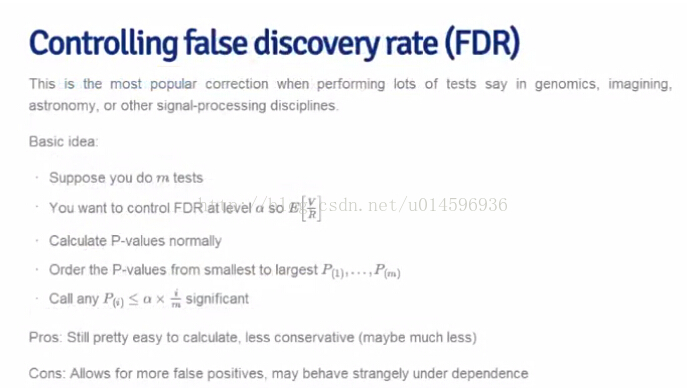
Controlling false discovery rate (FDR)

This is the most popular correction when performing lots of tests say in genomics, imaging, astronomy, or other signal-processing disciplines.

Basic idea:

• Suppose you do $m$ tests
• You want to control FDR at level $\alpha$ so $E\left[\frac{V}{R}\right]$
• Calculate P-values normally
• Order the P-values from smallest to largest $P_{(1)},...,P_{(m)}$
• Call any $P_{(i)} \leq \alpha \times \frac{i}{m}$ significant

Pros: Still pretty easy to calculate, less conservative (maybe much less)

Cons: Allows for more false positives, may behave strangely under dependence

Case study I: no true positives

set.seed(1010093)
pValues <- rep(NA,1000)
for(i in 1:1000){
  y <- rnorm(20)
  x <- rnorm(20)
  pValues[i] <- summary(lm(y ~ x))$coeff[2,4]
}

# Controls false positive rate
sum(pValues < 0.05)

[1] 51

---

Case study I: no true positives

# Controls FWER 
sum(p.adjust(pValues,method="bonferroni") < 0.05)

[1] 0

# Controls FDR 
sum(p.adjust(pValues,method="BH") < 0.05)

[1] 0

---

Case study II: 50% true positives

set.seed(1010093)
pValues <- rep(NA,1000)
for(i in 1:1000){
  x <- rnorm(20)
  # First 500 beta=0, last 500 beta=2
  if(i <= 500){y <- rnorm(20)}else{ y <- rnorm(20,mean=2*x)}
  pValues[i] <- summary(lm(y ~ x))$coeff[2,4]
}
trueStatus <- rep(c("zero","not zero"),each=500)
table(pValues < 0.05, trueStatus)

       trueStatus
        not zero zero
  FALSE        0  476
  TRUE       500   24

---

Case study II: 50% true positives

# Controls FWER 
table(p.adjust(pValues,method="bonferroni") < 0.05,trueStatus)

       trueStatus
        not zero zero
  FALSE       23  500
  TRUE       477    0

# Controls FDR 
table(p.adjust(pValues,method="BH") < 0.05,trueStatus)

       trueStatus
        not zero zero
  FALSE        0  487
  TRUE       500   13

---

Case study II: 50% true positives

P-values versus adjusted P-values

par(mfrow=c(1,2))
plot(pValues,p.adjust(pValues,method="bonferroni"),pch=19)
plot(pValues,p.adjust(pValues,method="BH"),pch=19)

---

Notes and resources

Notes:

• Multiple testing is an entire subfield
• A basic Bonferroni/BH correction is usually enough
• If there is strong dependence between tests there may be problems
  • Consider method="BY"

Further resources:

• Multiple testing procedures with applications to genomics
• Statistical significance for genome-wide studies
• Introduction to multiple testing

4.4 resampledInference 重取样推断

The jackknife

• The jackknife is a tool for estimating standard errors and the bias of estimators
• As its name suggests, the jackknife is a small, handy tool; in contrast to the bootstrap, which is then the moral equivalent of a giant workshop full of tools
• Both the jackknife and the bootstrap involve resampling data; that is, repeatedly creating new data sets from the original data

---

The jackknife

• The jackknife deletes each observation and calculates an estimate based on the remaining $n-1$ of them
• It uses this collection of estimates to do things like estimate the bias and the standard error
• Note that estimating the bias and having a standard error are not needed for things like sample means, which we know are unbiased estimates of population means and what their standard errors are

---

The jackknife

• We'll consider the jackknife for univariate data(单变量）
• Let $X_1,\ldots,X_n$ be a collection of data used to estimate a parameter $\theta$
• Let $\hat \theta$ be the estimate based on the full data set
• Let $\hat \theta_{i}$ be the estimate of $\theta$ obtained by deleting observation $i$
• Let $\bar \theta = \frac{1}{n}\sum_{i=1}^n \hat \theta_{i}$

---

Continued

• Then, the jackknife estimate of the bias is $$ (n - 1) \left(\bar \theta - \hat \theta\right) $$ (how far the average delete-one estimate is from the actual estimate)
• The jackknife estimate of the standard error is $$ \left[\frac{n-1}{n}\sum_{i=1}^n (\hat \theta_i - \bar\theta )^2\right]^{1/2} $$ (the deviance of the delete-one estimates from the average delete-one estimate)

---

Example

We want to estimate the bias and standard error of the median

library(UsingR)
data(father.son)
x <- father.son$sheight
n <- length(x)
theta <- median(x)
jk <- sapply(1 : n,
             function(i) median(x[-i])
             )
thetaBar <- mean(jk)
biasEst <- (n - 1) * (thetaBar - theta) 
seEst <- sqrt((n - 1) * mean((jk - thetaBar)^2))

---

Example

c(biasEst, seEst)

[1] 0.0000 0.1014

library(bootstrap)
temp <- jackknife(x, median)
c(temp$jack.bias, temp$jack.se)

[1] 0.0000 0.1014

---

Example

• Both methods (of course) yield an estimated bias of 0 and a se of 0.1014
• Odd little fact: the jackknife estimate of the bias for the median is always $0$ when the number of observations is even（偶数）
• It has been shown that the jackknife is a linear approximation to the bootstrap
• Generally do not use the jackknife for sample quantiles like the median; as it has been shown to have some poor properties

---

Pseudo observations

• Another interesting way to think about the jackknife uses pseudo observations
• Let $$ \mbox{Pseudo Obs} = n \hat \theta - (n - 1) \hat \theta_{i} $$
• Think of these as ``whatever observation $i$ contributes to the estimate of $\theta$''
• Note when $\hat \theta$ is the sample mean, the pseudo observations are the data themselves
• Then the sample standard error of these observations is the previous jackknife estimated standard error.
• The mean of these observations is a bias-corrected estimate of $\theta$

---

The bootstrap

• The bootstrap is a tremendously(异常) useful tool for constructing confidence intervals and calculating standard errors for difficult statistics
• For example, how would one derive a confidence interval for the median?
• The bootstrap procedure follows from the so called bootstrap principle

---

The bootstrap principle

• Suppose that I have a statistic that estimates some population parameter, but I don't know its sampling distribution
• The bootstrap principle suggests using the distribution defined by the data to approximate its sampling distribution

---

The bootstrap in practice

• In practice, the bootstrap principle is always carried out using simulation
• We will cover only a few aspects of bootstrap resampling

• The general procedure follows by first simulating complete data sets from the observed data with replacement

  • This is approximately drawing from the sampling distribution of that statistic, at least as far as the data is able to approximate the true population distribution

• Calculate the statistic for each simulated data set

• Use the simulated statistics to either define a confidence interval or take the standard deviation to calculate a standard error

---

Nonparametric bootstrap algorithm example

• Bootstrap procedure for calculating confidence interval for the median from a data set of $n$ observations

  i. Sample $n$ observations with replacement from the observed data resulting in one simulated complete data set

  ii. Take the median of the simulated data set

  iii. Repeat these two steps $B$ times, resulting in $B$ simulated medians

  iv. These medians are approximately drawn from the sampling distribution of the median of $n$ observations; therefore we can

  • Draw a histogram of them
  • Calculate their standard deviation to estimate the standard error of the median
  • Take the $2.5^{th}$ and $97.5^{th}$ percentiles as a confidence interval for the median

---

Example code

B <- 1000
resamples <- matrix(sample(x,
                           n * B,
                           replace = TRUE),
                    B, n)
medians <- apply(resamples, 1, median)
sd(medians)

[1] 0.08546

quantile(medians, c(.025, .975))

 2.5% 97.5% 
68.43 68.82 

---

Histogram of bootstrap resamples

hist(medians)

---

Notes on the bootstrap

• The bootstrap is non-parametric
• Better percentile bootstrap confidence intervals correct for bias
• There are lots of variations on bootstrap procedures; the book "An Introduction to the Bootstrap"" by Efron and Tibshirani is a great place to start for both bootstrap and jackknife information

---

Group comparisons

• Consider comparing two independent groups.
• Example, comparing sprays B and C

data(InsectSprays)
boxplot(count ~ spray, data = InsectSprays)

---

Permutation tests

• Consider the null hypothesis that the distribution of the observations from each group is the same
• Then, the group labels are irrelevant
• We then discard the group levels and permute the combined data
• Split the permuted data into two groups with $n_A$ and $n_B$ observations (say by always treating the first $n_A$ observations as the first group)
• Evaluate the probability of getting a statistic as large or large than the one observed
• An example statistic would be the difference in the averages between the two groups; one could also use a t-statistic

---

Variations on permutation testing

Data type	Statistic	Test name
Ranks	rank sum	rank sum test
Binary	hypergeometric prob	Fisher's exact test
Raw data		ordinary permutation test

• Also, so-called randomization tests are exactly permutation tests, with a different motivation.
• For matched data, one can randomize the signs
  • For ranks, this results in the signed rank test
• Permutation strategies work for regression as well
  • Permuting a regressor of interest
• Permutation tests work very well in multivariate settings

---

Permutation test for pesticide data

subdata <- InsectSprays[InsectSprays$spray %in% c("B", "C"),]
y <- subdata$count
group <- as.character(subdata$spray)
testStat <- function(w, g) mean(w[g == "B"]) - mean(w[g == "C"])
observedStat <- testStat(y, group)
permutations <- sapply(1 : 10000, function(i) testStat(y, sample(group)))
observedStat

[1] 13.25

mean(permutations > observedStat)

[1] 0

---

Histogram of permutations