霍夫变换（直线检测）

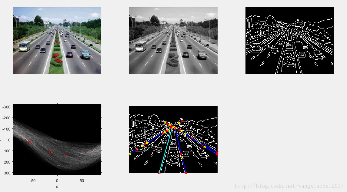
霍夫变换对于边缘检测来说是一个非常重要的工具，它可以通过连接技术将像素组合成完整的边缘。主要是通过图像空间与参数空间的转换。下面检测车道线图片。
霍夫变换的数学思想，将参数空间离散化，建立一个二维数组累加器A(a,b)=0，对每一个图像坐标系中的前景点（x,y）,都能在参数空间中算出一组A(a,b)，a=0,1,2,3,…,n，遍历完m个前景点后，生产m*n组A(a,b)，统计出现频率最高的几个点，就是图像坐标系中的线段（每一个点都是一条线段）

%通过霍夫变换检测车道线

I1 = imread('chedao.png');
I = rgb2gray(I1);
subplot(2,3,1);
imshow(I1);
subplot(2,3,2);
imshow(I);

%通过Canny算子检测边缘
BW = edge(I,'canny');
subplot(2,3,3);
imshow(BW);

%执行霍夫变换 显示霍夫矩阵
[H,T,R] = hough(BW);
subplot(2,3,4);
imshow(H,[],'XData',T,'YData',R,'InitialMagnification','fit');
xlabel('\theta'),ylabel('\rho');
axis on,axis normal,hold on;

%在霍夫矩阵中找到前五个大于最大值0.3倍的峰值
P = houghpeaks(H,5,'threshold',ceil(0.3*max(H(:))));
x = T(P(:,2));
y = R(P(:,1));
plot(x,y,'s','color','red');

%找到并绘制直线
%lines = houghlines(BW,T,R,P,'FillGap',1,'MinLength',100);
lines = houghlines(BW,T,R,P,'FillGap',5,'MinLength',5);
subplot(2,3,5);
imshow(BW),hold on;
max_len = 0;
for k = 1:length(lines)
    xy = [lines(k).point1;lines(k).point2];
    plot(xy(:,1),xy(:,2),'LineWidth',2,'Color','blue');

    %绘制线段端点
    plot(xy(1,1),xy(1,2),'x','LineWidth',2,'Color','yellow');
    plot(xy(2,1),xy(2,2),'x','LineWidth',2,'Color','red');

    % 确定最长线段
    len = norm(lines(k).point1-lines(k).point2);
    if (len > max_len)
        max_len = len;
        xy_long = xy;
    end
end

%高亮显示最长线段
plot(xy_long(:,1),xy_long(:,2),'LineWidth',2,'Color','cyan');