Python3-sklearn

最新推荐文章于 2024-08-02 11:14:12 发布

风吴痕

最新推荐文章于 2024-08-02 11:14:12 发布

阅读量4.5k

点赞数

分类专栏： sklearn 文章标签： sklearn

sklearn 专栏收录该内容

3 篇文章 0 订阅

订阅专栏

参考地址：

1、http://www.scipy-lectures.org/packages/scikit-learn/index.html

2、http://scikit-learn.org/stable/

3.6. scikit-learn: machine learning in Python

3.6.1. Introduction: problem settings

3.6.1.1. What is machine learning?

../../_images/sphx_glr_plot_separator_001.png

A classification proble

../../_images/sphx_glr_plot_linear_regression_001.png

A regression problem

3.6.1.2. Data in scikit-learn

The data matrix

two-dimensional array or matrix [n_samples, n_features]

n_samples: The number of samples

n_features: The number of features or distinct traits that can be used to describe each item in a quantitative manner.

A Simple Example: the Iris Dataset

The application problem

As an example of a simple dataset, let us a look at the iris data stored by scikit-learn. Suppose we want to recognize species of irises. The data consists of measurements of threedifferent species of irises:


Setosa Iris	Versicolor Iris	Virginica Iris

Quick Question:

If we want to design an algorithm to recognize iris species, what might the data be?

Remember: we need a 2D array of size [n_samples x n_features].

What would the n_samples refer to?
What might the n_features refer to?

Remember that there must be a fixed number of features for each sample, and feature number i must be a similar kind of quantity for each sample.

Loading the Iris Data with Scikit-learn

Scikit-learn has a very straightforward set of data on these iris species. The data consist of the following:

Features in the Iris dataset:
- sepal length (cm)
- sepal width (cm)
- petal length (cm)
- petal width (cm)
Target classes to predict:
- Setosa
- Versicolour
- Virginica

scikit-learn embeds a copy of the iris CSV file along with a function to load it into numpy arrays:

 
   >>> 
   >>> from sklearn.datasets import load_iris
>>> iris = load_iris()

Note

Import sklearn Note that scikit-learn is imported as sklearn

The features of each sample flower are stored in the data attribute of the dataset:

 
   >>> 
   >>> print(iris.data.shape)
(150, 4)
>>> n_samples, n_features = iris.data.shape
>>> print(n_samples)
150
>>> print(n_features)
4
>>> print(iris.data[0])
[ 5.1  3.5  1.4  0.2]
 
  

The information about the class of each sample is stored in the targetattribute of the dataset:

 
   >>> 
   >>> print(iris.target.shape)
(150,)
>>> print(iris.target)
[0 0 0 0 0 0 0 0 0 0 0 0 0 0 0 0 0 0 0 0 0 0 0 0 0 0 0 0 0 0 0 0 0 0 0 0 0
 0 0 0 0 0 0 0 0 0 0 0 0 0 1 1 1 1 1 1 1 1 1 1 1 1 1 1 1 1 1 1 1 1 1 1 1 1
 1 1 1 1 1 1 1 1 1 1 1 1 1 1 1 1 1 1 1 1 1 1 1 1 1 1 2 2 2 2 2 2 2 2 2 2 2
 2 2 2 2 2 2 2 2 2 2 2 2 2 2 2 2 2 2 2 2 2 2 2 2 2 2 2 2 2 2 2 2 2 2 2 2 2
 2 2]
 
  

The names of the classes are stored in the last attribute, namelytarget_names:

 
   >>> 
   >>> print(iris.target_names)
['setosa' 'versicolor' 'virginica']

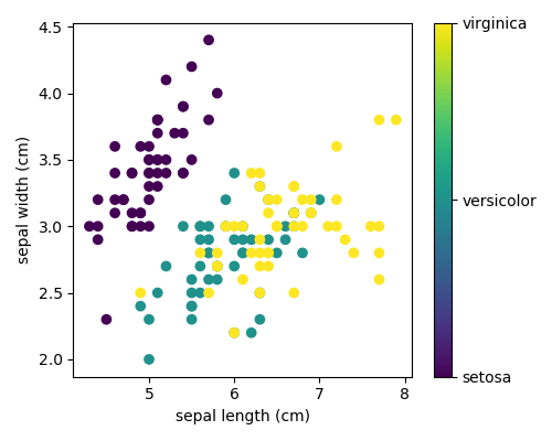
This data is four-dimensional, but we can visualize two of the dimensions at a time using a scatter plot:

../../_images/sphx_glr_plot_iris_scatter_001.png

Excercise:

Can you choose 2 features to find a plot where it is easier to seperate the different classes of irises?

Hint: click on the figure above to see the code that generates it, and modify this code.

3.6.2. Basic principles of machine learning with scikit-learn

3.6.2.1. Introducing the scikit-learn estimator object

Every algorithm is exposed in scikit-learn via an ‘’Estimator’’ object. For instance a linear regression is:sklearn.linear_model.LinearRegression

 
    >>> 
    >>> from sklearn.linear_model import LinearRegression

Estimator parameters: All the parameters of an estimator can be set when it is instantiated:

 
    >>> 
    >>> model = LinearRegression(normalize=True)
>>> print(model.normalize)
True
>>> print(model)
LinearRegression(copy_X=True, fit_intercept=True, n_jobs=1, normalize=True)
 
   

Fitting on data

Let’s create some simple data with numpy:

 
     >>> 
     >>> import numpy as np
>>> x = np.array([0, 1, 2])
>>> y = np.array([0, 1, 2])

>>> X = x[:, np.newaxis] # The input data for sklearn is 2D: (samples == 3 x features == 1)
>>> X
array([[0],
       [1],
       [2]])

>>> model.fit(X, y)
LinearRegression(copy_X=True, fit_intercept=True, n_jobs=1, normalize=True)
 
    

Estimated parameters: When data is fitted with an estimator, parameters are estimated from the data at hand. All the estimated parameters are attributes of the estimator object ending by an underscore:

 
     >>> 
     >>> model.coef_
array([ 1.]) 
    

from sklearn.linear_model import LinearRegression

model = LinearRegression(normalize=True)
print(model.normalize)

print(model)

import numpy as np
x = np.array([0, 1, 2])
y = np.array([0, 1, 2])

X = x[:, np.newaxis] # The input data for sklearn is 2D: (samples == 3 x features == 1)

model.fit(X, y) # model.fit(X, y[:,np.newaxis])

print(model.coef_) # Estimated parameters  y=(model.coef_)*x

print(model.predict(np.array([3,4,5])[:, np.newaxis])) # [ 3.  4.  5.]

3.6.2.2. Supervised Learning: Classification and regression

Classification : K nearest neighbors (kNN) is one of the simplest learning strategies

 
   from sklearn import neighbors, datasets
iris = datasets.load_iris()
X, y = iris.data, iris.target
knn = neighbors.KNeighborsClassifier(n_neighbors=1)
knn.fit(X, y)
# What kind of iris has 3cm x 5cm sepal and 4cm x 2cm petal?
print(iris.target_names[knn.predict([[3, 5, 4, 2]])])
 
  

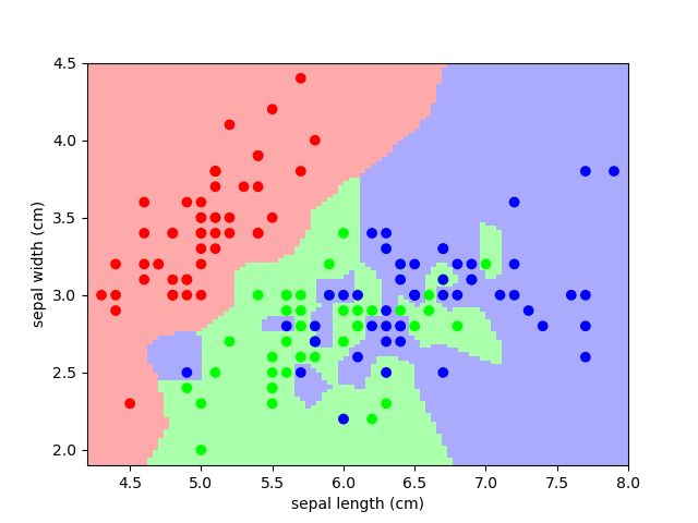
../../_images/sphx_glr_plot_iris_knn_001.png

A plot of the sepal space and the prediction of the KNN

from sklearn import neighbors, datasets
iris = datasets.load_iris()
X, y = iris.data, iris.target
knn = neighbors.KNeighborsClassifier(n_neighbors=5)
knn.fit(X, y)
# What kind of iris has 3cm x 5cm sepal and 4cm x 2cm petal?
print(iris.target_names[knn.predict([[3, 5, 4, 2]])]) # ['versicolor']
print(knn.score(X,y)) # 0.966666666667
print(knn.predict_proba([[3, 5, 4, 2]])) # [[ 0.   0.8  0.2]]
print(knn.predict([[3, 5, 4, 2]])) # [1]

Regression: The simplest possible regression setting is the linear regressionone:

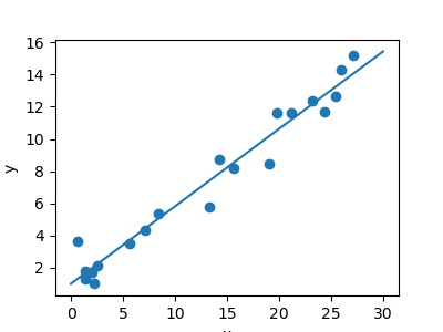
A plot of a simple linear regression.

3.6.2.3. A recap on Scikit-learn’s estimator interface

In all Estimators:
	`model.fit()` : fit training data. For supervised learning applications, this accepts two arguments: the data `X` and the labels `y` (e.g.`model.fit(X, y)`). For unsupervised learning applications, this accepts only a single argument, the data `X` (e.g. `model.fit(X)`).
In supervised estimators:
	`model.predict()` : given a trained model, predict the label of a new set of data. This method accepts one argument, the new data `X_new`(e.g. `model.predict(X_new)`), and returns the learned label for each object in the array. `model.predict_proba()` : For classification problems, some estimators also provide this method, which returns the probability that a new observation has each categorical label. In this case, the label with the highest probability is returned by `model.predict()`. `model.score()` : for classification or regression problems, most (all?) estimators implement a score method. Scores are between 0 and 1, with a larger score indicating a better fit.
In unsupervised estimators:
	`model.transform()` : given an unsupervised model, transform new data into the new basis. This also accepts one argument `X_new`, and returns the new representation of the data based on the unsupervised model. `model.fit_transform()` : some estimators implement this method, which more efficiently performs a fit and a transform on the same input data.

3.6.2.4. Regularization: what it is and why it is necessary

3.6.3. Supervised Learning: Classification of Handwritten Digits

3.6.3.1. The nature of the data

from sklearn.datasets import load_digits
>>> digits = load_digits()

# plot the digits: each image is 8x8 pixels
for i in range(64):
    ax = fig.add_subplot(8, 8, i + 1, xticks=[], yticks=[])
    ax.imshow(digits.images[i], cmap=plt.cm.binary, interpolation='nearest')

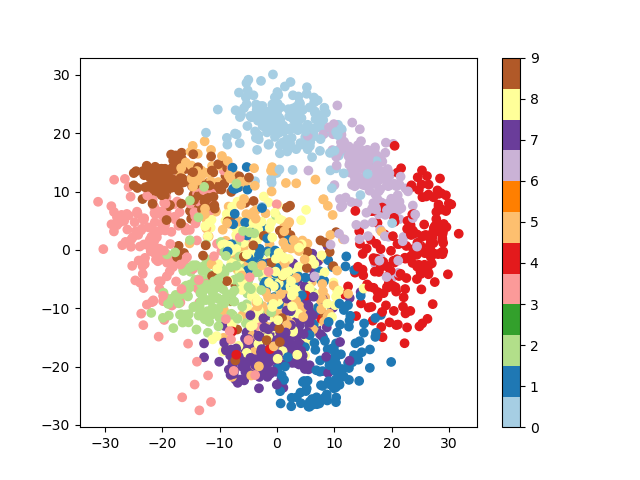
3.6.3.2. Visualizing the Data on its principal components

from sklearn.decomposition import PCA
>>> pca = PCA(n_components=2)
>>> proj = pca.fit_transform(digits.data)
>>> plt.scatter(proj[:, 0], proj[:, 1], c=digits.target) 
<matplotlib.collections.PathCollection object at ...>
>>> plt.colorbar() 
<matplotlib.colorbar.Colorbar object at ...>

We’ll start with the most straightforward one, Principal Component Analysis (PCA) .

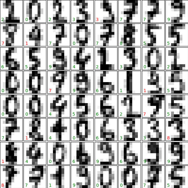
3.6.3.3. Gaussian Naive Bayes Classification

One good method to keep in mind is Gaussian Naive Bayes ( sklearn.naive_bayes.GaussianNB )

from sklearn.naive_bayes import GaussianNB
>>> from sklearn.model_selection import train_test_split

>>> # split the data into training and validation sets
>>> X_train, X_test, y_train, y_test = train_test_split(digits.data, digits.target)

>>> # train the model
>>> clf = GaussianNB()
>>> clf.fit(X_train, y_train)
GaussianNB(priors=None)

>>> # use the model to predict the labels of the test data
>>> predicted = clf.predict(X_test)
>>> expected = y_test
>>> print(predicted) 
[1 7 7 7 8 2 8 0 4 8 7 7 0 8 2 3 5 8 5 3 7 9 6 2 8 2 2 7 3 5...]
>>> print(expected) 
[1 0 4 7 8 2 2 0 4 3 7 7 0 8 2 3 4 8 5 3 7 9 6 3 8 2 2 9 3 5...]

from sklearn.naive_bayes import GaussianNB
from sklearn.model_selection import train_test_split
from sklearn.datasets import load_digits
digits = load_digits()

# split the data into training and validation sets
X_train, X_test, y_train, y_test = train_test_split(digits.data, digits.target)

# train the model
clf = GaussianNB()
clf.fit(X_train, y_train)


# use the model to predict the labels of the test data
predicted = clf.predict(X_test)
expected = y_test
# print(predicted)

# print(expected)

print(clf.score(X_test, y_test)) # 0.871111111111

from sklearn.decomposition import PCA
import matplotlib.pyplot as plt
pca = PCA(n_components=5)
proj = pca.fit_transform(digits.data)

plt.scatter(proj[:, 0], proj[:, 1], c=digits.target)

plt.colorbar()

plt.show()

3.6.3.4. Quantitative Measurement of Performance

matches = (predicted == expected)
>>> print(matches.sum())
367
>>> print(len(matches))
450
>>> matches.sum() / float(len(matches))
0.81555555555555559

But there are other more sophisticated metrics that can be used to judge the performance of a classifier: several are available in the sklearn.metrics submodule.

 
   from sklearn import metrics
>>> print(metrics.classification_report(expected, predicted))
             precision    recall  f1-score   support

          0       1.00      0.91      0.95        46
          1       0.76      0.64      0.69        44
          2       0.85      0.62      0.72        47
          3       0.98      0.82      0.89        49
          4       0.89      0.86      0.88        37
          5       0.97      0.93      0.95        41
          6       1.00      0.98      0.99        44
          7       0.73      1.00      0.84        45
          8       0.50      0.90      0.64        49
          9       0.93      0.54      0.68        48

avg / total       0.86      0.82      0.82       450
 
  

 
   print(metrics.confusion_matrix(expected, predicted))
[[42  0  0  0  3  0  0  1  0  0]
 [ 0 28  0  0  0  0  0  1 13  2]
 [ 0  3 29  0  0  0  0  0 15  0]
 [ 0  0  2 40  0  0  0  2  5  0]
 [ 0  0  1  0 32  1  0  3  0  0]
 [ 0  0  0  0  0 38  0  2  1  0]
 [ 0  0  1  0  0  0 43  0  0  0]
 [ 0  0  0  0  0  0  0 45  0  0]
 [ 0  3  1  0  0  0  0  1 44  0]
 [ 0  3  0  1  1  0  0  7 10 26]]
 
  

We see here that in particular, the numbers 1, 2, 3, and 9 are often being labeled 8.

3.6.4. Supervised Learning: Regression of Housing Data

3.6.4.1. A quick look at the data

from sklearn.datasets import load_boston
>>> data = load_boston()
>>> print(data.data.shape)
(506, 13)
>>> print(data.target.shape)
(506,)

print(data.DESCR) 
Boston House Prices dataset
===========================

Notes
------
Data Set Characteristics:

    :Number of Instances: 506

    :Number of Attributes: 13 numeric/categorical predictive

    :Median Value (attribute 14) is usually the target

    :Attribute Information (in order):
        - CRIM     per capita crime rate by town
        - ZN       proportion of residential land zoned for lots over 25,000 sq.ft.
        - INDUS    proportion of non-retail business acres per town
        - CHAS     Charles River dummy variable (= 1 if tract bounds river; 0 otherwise)
        - NOX      nitric oxides concentration (parts per 10 million)
        - RM       average number of rooms per dwelling
        - AGE      proportion of owner-occupied units built prior to 1940
        - DIS      weighted distances to five Boston employment centres
        - RAD      index of accessibility to radial highways
        - TAX      full-value property-tax rate per $10,000
        - PTRATIO  pupil-teacher ratio by town
        - B        1000(Bk - 0.63)^2 where Bk is the proportion of blacks by town
        - LSTAT    % lower status of the population
        - MEDV     Median value of owner-occupied homes in $1000's
...

 
   plt.hist(data.target)  
(array([...

../../_images/sphx_glr_plot_boston_prediction_001.png

for index, feature_name in enumerate(data.feature_names):
...     plt.figure()
...     plt.scatter(data.data[:, index], data.target)  
<matplotlib.figure.Figure object...

3.6.4.2. Predicting Home Prices: a Simple Linear Regression

from sklearn.model_selection import train_test_split
>>> X_train, X_test, y_train, y_test = train_test_split(data.data, data.target)
>>> from sklearn.linear_model import LinearRegression
>>> clf = LinearRegression()
>>> clf.fit(X_train, y_train)
LinearRegression(copy_X=True, fit_intercept=True, n_jobs=1, normalize=False)
>>> predicted = clf.predict(X_test)
>>> expected = y_test
>>> print("RMS: %s" % np.sqrt(np.mean((predicted - expected) ** 2))) 
RMS: 5.0059...

Exercise: Gradient Boosting Tree Regression

There are many other types of regressors available in scikit-learn: we’ll try a more powerful one here.

Use the GradientBoostingRegressor class to fit the housing data.

hint You can copy and paste some of the above code, replacingLinearRegression with GradientBoostingRegressor:

 
   from sklearn.ensemble import GradientBoostingRegressor
# Instantiate the model, fit the results, and scatter in vs. out

Solution The solution is found in the code of this chapter

3.6.5. Measuring prediction performance

3.6.5.1. A quick test on the K-neighbors classifier

 
   # Get the data
>>> from sklearn.datasets import load_digits
>>> digits = load_digits()
>>> X = digits.data
>>> y = digits.target

>>> # Instantiate and train the classifier
>>> from sklearn.neighbors import KNeighborsClassifier
>>> clf = KNeighborsClassifier(n_neighbors=1)
>>> clf.fit(X, y) 
KNeighborsClassifier(...)

>>> # Check the results using metrics
>>> from sklearn import metrics
>>> y_pred = clf.predict(X)

>>> print(metrics.confusion_matrix(y_pred, y))
[[178   0   0   0   0   0   0   0   0   0]
 [  0 182   0   0   0   0   0   0   0   0]
 [  0   0 177   0   0   0   0   0   0   0]
 [  0   0   0 183   0   0   0   0   0   0]
 [  0   0   0   0 181   0   0   0   0   0]
 [  0   0   0   0   0 182   0   0   0   0]
 [  0   0   0   0   0   0 181   0   0   0]
 [  0   0   0   0   0   0   0 179   0   0]
 [  0   0   0   0   0   0   0   0 174   0]
 [  0   0   0   0   0   0   0   0   0 180]]
 
  

from sklearn.datasets import load_boston
>>> from sklearn.tree import DecisionTreeRegressor

>>> data = load_boston()
>>> clf = DecisionTreeRegressor().fit(data.data, data.target)
>>> predicted = clf.predict(data.data)
>>> expected = data.target

>>> plt.scatter(expected, predicted) 
<matplotlib.collections.PathCollection object at ...>
>>> plt.plot([0, 50], [0, 50], '--k') 
[<matplotlib.lines.Line2D object at ...]

3.6.5.2. A correct approach: Using a validation set

In scikit-learn such a random split can be quickly computed with the train_test_split() function:

 
   from sklearn import model_selection
>>> X = digits.data
>>> y = digits.target

>>> X_train, X_test, y_train, y_test = model_selection.train_test_split(X, y,
...                                         test_size=0.25, random_state=0)

>>> print("%r, %r, %r" % (X.shape, X_train.shape, X_test.shape))
(1797, 64), (1347, 64), (450, 64)

Now we train on the training data, and test on the testing data:

 
   >>> 
   >>> clf = KNeighborsClassifier(n_neighbors=1).fit(X_train, y_train)
>>> y_pred = clf.predict(X_test)

>>> print(metrics.confusion_matrix(y_test, y_pred))
[[37  0  0  0  0  0  0  0  0  0]
 [ 0 43  0  0  0  0  0  0  0  0]
 [ 0  0 43  1  0  0  0  0  0  0]
 [ 0  0  0 45  0  0  0  0  0  0]
 [ 0  0  0  0 38  0  0  0  0  0]
 [ 0  0  0  0  0 47  0  0  0  1]
 [ 0  0  0  0  0  0 52  0  0  0]
 [ 0  0  0  0  0  0  0 48  0  0]
 [ 0  0  0  0  0  0  0  0 48  0]
 [ 0  0  0  1  0  1  0  0  0 45]]
>>> print(metrics.classification_report(y_test, y_pred))
             precision    recall  f1-score   support

          0       1.00      1.00      1.00        37
          1       1.00      1.00      1.00        43
          2       1.00      0.98      0.99        44
          3       0.96      1.00      0.98        45
          4       1.00      1.00      1.00        38
          5       0.98      0.98      0.98        48
          6       1.00      1.00      1.00        52
          7       1.00      1.00      1.00        48
          8       1.00      1.00      1.00        48
          9       0.98      0.96      0.97        47

avg / total       0.99      0.99      0.99       450 
  

metrics.f1_score(y_test, y_pred, average="macro") 
0.991367...

metrics.f1_score(y_train, clf.predict(X_train), average="macro")
1.0

3.6.5.3. Model Selection via Validation

from sklearn.naive_bayes import GaussianNB
>>> from sklearn.neighbors import KNeighborsClassifier
>>> from sklearn.svm import LinearSVC

>>> X = digits.data
>>> y = digits.target
>>> X_train, X_test, y_train, y_test = model_selection.train_test_split(X, y,
...                             test_size=0.25, random_state=0)

>>> for Model in [GaussianNB, KNeighborsClassifier, LinearSVC]:
...     clf = Model().fit(X_train, y_train)
...     y_pred = clf.predict(X_test)
...     print('%s: %s' %
...           (Model.__name__, metrics.f1_score(y_test, y_pred, average="macro")))  
GaussianNB: 0.8332741681...
KNeighborsClassifier: 0.9804562804...
LinearSVC: 0.93...

For LinearSVC , use loss='l2' and loss='l1' . For KNeighborsClassifier we use n_neighbors between 1 and 10. Note that GaussianNB does not have any adjustable hyperparameters.

 
   LinearSVC(loss='l1'): 0.930570687535
LinearSVC(loss='l2'): 0.933068826918
-------------------
KNeighbors(n_neighbors=1): 0.991367521884
KNeighbors(n_neighbors=2): 0.984844206884
KNeighbors(n_neighbors=3): 0.986775344954
KNeighbors(n_neighbors=4): 0.980371905382
KNeighbors(n_neighbors=5): 0.980456280495
KNeighbors(n_neighbors=6): 0.975792419414
KNeighbors(n_neighbors=7): 0.978064579214
KNeighbors(n_neighbors=8): 0.978064579214
KNeighbors(n_neighbors=9): 0.978064579214
KNeighbors(n_neighbors=10): 0.975555089773
 
  

Solution: code source

3.6.5.4. Cross-validation

clf = KNeighborsClassifier()
>>> from sklearn.model_selection import cross_val_score
>>> cross_val_score(clf, X, y, cv=5)
array([ 0.9478022 ,  0.9558011 ,  0.96657382,  0.98039216,  0.96338028])

from sklearn.model_selection import ShuffleSplit
>>> cv = ShuffleSplit(n_splits=5)
>>> cross_val_score(clf, X, y, cv=cv)  
array([...])

There exists many different cross-validation strategies in scikit-learn. They are often useful to take in account non iid datasets.

3.6.5.5. Hyperparameter optimization with cross-validation

from sklearn.datasets import load_diabetes
>>> data = load_diabetes()
>>> X, y = data.data, data.target
>>> print(X.shape)
(442, 10)

from sklearn.linear_model import Ridge, Lasso

>>> for Model in [Ridge, Lasso]:
...     model = Model()
...     print('%s: %s' % (Model.__name__, cross_val_score(model, X, y).mean()))
Ridge: 0.409427438303
Lasso: 0.353800083299

Basic Hyperparameter Optimization

alphas = np.logspace(-3, -1, 30)

>>> for Model in [Lasso, Ridge]:
...     scores = [cross_val_score(Model(alpha), X, y, cv=3).mean()
...               for alpha in alphas]
...     plt.plot(alphas, scores, label=Model.__name__) 
[<matplotlib.lines.Line2D object at ...

Automatically Performing Grid Search

sklearn.grid_search.GridSearchCV is constructed with an estimator, as well as a dictionary of parameter values to be searched. We can find the optimal parameters this way:

from sklearn.grid_search import GridSearchCV
>>> for Model in [Ridge, Lasso]:
...     gscv = GridSearchCV(Model(), dict(alpha=alphas), cv=3).fit(X, y)
...     print('%s: %s' % (Model.__name__, gscv.best_params_))
Ridge: {'alpha': 0.062101694189156162}
Lasso: {'alpha': 0.01268961003167922}

Built-in Hyperparameter Search

from sklearn.linear_model import RidgeCV, LassoCV
>>> for Model in [RidgeCV, LassoCV]:
...     model = Model(alphas=alphas, cv=3).fit(X, y)
...     print('%s: %s' % (Model.__name__, model.alpha_))
RidgeCV: 0.0621016941892
LassoCV: 0.0126896100317

Nested cross-validation

for Model in [RidgeCV, LassoCV]:
    scores = cross_val_score(Model(alphas=alphas, cv=3), X, y, cv=3)
    print(Model.__name__, np.mean(scores))

3.6.6. Unsupervised Learning: Dimensionality Reduction and Visualization

3.6.6.1. Dimensionality Reduction: PCA

We’ll use sklearn.decomposition.PCA on the iris dataset:

 
   >>> 
   >>> X = iris.data
>>> y = iris.target 
  

 
   from sklearn.decomposition import PCA
>>> pca = PCA(n_components=2, whiten=True)
>>> pca.fit(X) 
PCA(..., n_components=2, ...)

Once fitted, PCA exposes the singular vectors in the components_ attribute:

 
   >>> 
   >>> pca.components_     
array([[ 0.36158..., -0.08226...,  0.85657...,  0.35884...],
       [ 0.65653...,  0.72971..., -0.17576..., -0.07470...]])

Other attributes are available as well:

 
   >>> 
   >>> pca.explained_variance_ratio_    
array([ 0.92461...,  0.05301...])

Let us project the iris dataset along those first two dimensions::

 
   >>> 
   >>> X_pca = pca.transform(X)
>>> X_pca.shape
(150, 2) 
  

X_pca.mean(axis=0) 
array([ ...e-15,  ...e-15])
>>> X_pca.std(axis=0)
array([ 1.,  1.])

3.6.6.2. Visualization with a non-linear embedding: tSNE

sklearn.manifold.TSNE is such a powerful manifold learning method.

# Take the first 500 data points: it's hard to see 1500 points
>>> X = digits.data[:500]
>>> y = digits.target[:500]

>>> # Fit and transform with a TSNE
>>> from sklearn.manifold import TSNE
>>> tsne = TSNE(n_components=2, random_state=0)
>>> X_2d = tsne.fit_transform(X)

>>> # Visualize the data
>>> plt.scatter(X_2d[:, 0], X_2d[:, 1], c=y) 
<matplotlib.collections.PathCollection object at ...>

3.6.7. The eigenfaces example: chaining PCA and SVMs

from sklearn import datasets
faces = datasets.fetch_olivetti_faces()
faces.data.shape

from matplotlib import pyplot as plt
fig = plt.figure(figsize=(8, 6))
# plot several images
for i in range(15):
    ax = fig.add_subplot(3, 5, i + 1, xticks=[], yticks=[])
    ax.imshow(faces.images[i], cmap=plt.cm.bone)

from sklearn.model_selection import train_test_split
X_train, X_test, y_train, y_test = train_test_split(faces.data,
        faces.target, random_state=0)

print(X_train.shape, X_test.shape)

3.6.7.1. Preprocessing: Principal Component Analysis

from sklearn import decomposition
pca = decomposition.PCA(n_components=150, whiten=True)
pca.fit(X_train)

plt.imshow(pca.mean_.reshape(faces.images[0].shape),
           cmap=plt.cm.bone)

print(pca.components_.shape)

fig = plt.figure(figsize=(16, 6))
for i in range(30):
    ax = fig.add_subplot(3, 10, i + 1, xticks=[], yticks=[])
    ax.imshow(pca.components_[i].reshape(faces.images[0].shape),
              cmap=plt.cm.bone)

 
   X_train_pca = pca.transform(X_train)
X_test_pca = pca.transform(X_test)
print(X_train_pca.shape)

Out:

 
   (300, 150)

 
   print(X_test_pca.shape)

Out:

 
   (100, 150) 
  

3.6.7.2. Doing the Learning: Support Vector Machines

from sklearn import svm
clf = svm.SVC(C=5., gamma=0.001)
clf.fit(X_train_pca, y_train)

import numpy as np
fig = plt.figure(figsize=(8, 6))
for i in range(15):
    ax = fig.add_subplot(3, 5, i + 1, xticks=[], yticks=[])
    ax.imshow(X_test[i].reshape(faces.images[0].shape),
              cmap=plt.cm.bone)
    y_pred = clf.predict(X_test_pca[i, np.newaxis])[0]
    color = ('black' if y_pred == y_test[i] else 'red')
    ax.set_title(faces.target[y_pred],
                 fontsize='small', color=color)

from sklearn import metrics
y_pred = clf.predict(X_test_pca)
print(metrics.classification_report(y_test, y_pred))

print(metrics.confusion_matrix(y_test, y_pred))

3.6.7.3. Pipelining

from sklearn.pipeline import Pipeline
clf = Pipeline([('pca', decomposition.PCA(n_components=150, whiten=True)),
                ('svm', svm.LinearSVC(C=1.0))])

clf.fit(X_train, y_train)

y_pred = clf.predict(X_test)
print(metrics.confusion_matrix(y_pred, y_test))

from sklearn import datasets
faces = datasets.fetch_olivetti_faces()
# faces.data(400,64*64)  faces.target(400,)

from matplotlib import pyplot as plt
fig = plt.figure(figsize=(8, 6))
# plot several images
for i in range(15):
    ax = fig.add_subplot(3, 5, i + 1, xticks=[], yticks=[])
    ax.imshow(faces.images[i], cmap=plt.cm.bone)
plt.show()


from sklearn.model_selection import train_test_split
X_train, X_test, y_train, y_test = train_test_split(faces.data,
        faces.target, random_state=0)

print(X_train.shape, X_test.shape) # (300, 4096) (100, 4096)


""" 方式一
from sklearn import decomposition
pca = decomposition.PCA(n_components=150, whiten=True) # 经过pca处理只保留150个特征
pca.fit(X_train)
'''

plt.imshow(pca.mean_.reshape(faces.images[0].shape),
           cmap=plt.cm.bone)

print(pca.components_.shape) # (150, 4096)

fig = plt.figure(figsize=(16, 6))
for i in range(30):
    ax = fig.add_subplot(3, 10, i + 1, xticks=[], yticks=[])
    ax.imshow(pca.components_[i].reshape(faces.images[0].shape),
              cmap=plt.cm.bone)
'''
# 数据进行pca处理
X_train_pca = pca.transform(X_train)
X_test_pca = pca.transform(X_test)
print(X_train_pca.shape) # (300, 150)
print(X_test_pca.shape) # (100, 150)

from sklearn import svm
clf = svm.SVC(C=5., gamma=0.001)
clf.fit(X_train_pca, y_train)

import numpy as np
fig = plt.figure(figsize=(8, 6))
for i in range(15):
    ax = fig.add_subplot(3, 5, i + 1, xticks=[], yticks=[])
    ax.imshow(X_test[i].reshape(faces.images[0].shape),
              cmap=plt.cm.bone)
    y_pred = clf.predict(X_test_pca[i, np.newaxis])[0]
    color = ('black' if y_pred == y_test[i] else 'red')
    ax.set_title(faces.target[y_pred],
                 fontsize='small', color=color)


from sklearn import metrics
y_pred = clf.predict(X_test_pca)
print(metrics.classification_report(y_test, y_pred))

print(metrics.confusion_matrix(y_test, y_pred))

# 使用原始数据
clf2 = svm.SVC(C=5., gamma=0.001)
clf2.fit(X_train, y_train)
y_pred2 = clf2.predict(X_test)
print(metrics.classification_report(y_test, y_pred2))
"""

# 方式一的简化版
from sklearn import decomposition
from sklearn import svm
from sklearn.pipeline import Pipeline
from sklearn import metrics
clf = Pipeline([('pca', decomposition.PCA(n_components=150, whiten=True)),
                ('svm', svm.LinearSVC(C=1.0))])

clf.fit(X_train, y_train)

y_pred = clf.predict(X_test)
print(metrics.classification_report(y_test, y_pred))
print(metrics.confusion_matrix(y_pred, y_test))
print(clf.score(X_test,y_test)) # 0.92

3.6.8. Parameter selection, Validation, and Testing

3.6.8.1. Hyperparameters, Over-fitting, and Under-fitting

We’ll explore a simple linear regression problem, withsklearn.linear_model.

 
   X = np.c_[ .5, 1].T
y = [.5, 1]
X_test = np.c_[ 0, 2].T

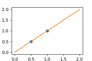
Without noise, as linear regression fits the data perfectly

 
   from sklearn import linear_model
regr = linear_model.LinearRegression()
regr.fit(X, y)
plt.plot(X, y, 'o')
plt.plot(X_test, regr.predict(X_test)) 
  

np.random.seed(0)
for _ in range(6):
    noisy_X = X + np.random.normal(loc=0, scale=.1, size=X.shape)
    plt.plot(noisy_X, y, 'o')
    regr.fit(noisy_X, y)
    plt.plot(X_test, regr.predict(X_test))

regr = linear_model.Ridge(alpha=.1)
np.random.seed(0)
for _ in range(6):
    noisy_X = X + np.random.normal(loc=0, scale=.1, size=X.shape)
    plt.plot(noisy_X, y, 'o')
    regr.fit(noisy_X, y)
    plt.plot(X_test, regr.predict(X_test))

plt.show()

3.6.8.2. Visualizing the Bias/Variance Tradeoff

Polynomial regression with scikit-learn

A polynomial regression is built by pipelining PolynomialFeatures and aLinearRegression:

 
   >>> 
   >>> from sklearn.pipeline import make_pipeline
>>> from sklearn.preprocessing import PolynomialFeatures
>>> from sklearn.linear_model import LinearRegression
>>> model = make_pipeline(PolynomialFeatures(degree=2), LinearRegression()) 
  

Validation Curves

Let us create a dataset like in the example above:

 
   >>> 
   >>> def generating_func(x, err=0.5):
...     return np.random.normal(10 - 1. / (x + 0.1), err)

>>> # randomly sample more data
>>> np.random.seed(1)
>>> x = np.random.random(size=200)
>>> y = generating_func(x, err=1.) 
  

We use sklearn.model_selection.validation_curve() tocompute train and test error, and plot it:

 
   >>> 
   >>> from sklearn.model_selection import validation_curve

>>> degrees = np.arange(1, 21)

>>> model = make_pipeline(PolynomialFeatures(), LinearRegression())

>>> # Vary the "degrees" on the pipeline step "polynomialfeatures"
>>> train_scores, validation_scores = validation_curve(
...                 model, x[:, np.newaxis], y,
...                 param_name='polynomialfeatures__degree',
...                 param_range=degrees)

>>> # Plot the mean train score and validation score across folds
>>> plt.plot(degrees, validation_scores.mean(axis=1), label='cross-validation')  
[<matplotlib.lines.Line2D object at ...>]
>>> plt.plot(degrees, train_scores.mean(axis=1), label='training')  
[<matplotlib.lines.Line2D object at ...>]
>>> plt.legend(loc='best')  
<matplotlib.legend.Legend object at ...> 
  

Learning Curves

scikit-learn provides sklearn.model_selection.learning_curve():

 
   >>> 
   >>> from sklearn.model_selection import learning_curve
>>> train_sizes, train_scores, validation_scores = learning_curve(
...     model, x[:, np.newaxis], y, train_sizes=np.logspace(-1, 0, 20))

>>> # Plot the mean train score and validation score across folds
>>> plt.plot(train_sizes, validation_scores.mean(axis=1), label='cross-validation') 
[<matplotlib.lines.Line2D object at ...>]
>>> plt.plot(train_sizes, train_scores.mean(axis=1), label='training') 
[<matplotlib.lines.Line2D object at ...>] 
  

3.6.8.3. Summary on model selection

High Bias

If a model shows high bias, the following actions might help:

Add more features. In our example of predicting home prices, it may be helpful to make use of information such as the neighborhood the house is in, the year the house was built, the size of the lot, etc. Adding these features to the training and test sets can improve a high-bias estimator
Use a more sophisticated model. Adding complexity to the model can help improve on bias. For a polynomial fit, this can be accomplished by increasing the degree d. Each learning technique has its own methods of adding complexity.
Use fewer samples. Though this will not improve the classification, a high-bias algorithm can attain nearly the same error with a smaller training sample. For algorithms which are computationally expensive, reducing the training sample size can lead to very large improvements in speed.
Decrease regularization. Regularization is a technique used to impose simplicity in some machine learning models, by adding a penalty term that depends on the characteristics of the parameters. If a model has high bias, decreasing the effect of regularization can lead to better results.

High Variance

If a model shows high variance, the following actions might help:

Use fewer features. Using a feature selection technique may be useful, and decrease the over-fitting of the estimator.
Use a simpler model. Model complexity and over-fitting go hand-in-hand.
Use more training samples. Adding training samples can reduce the effect of over-fitting, and lead to improvements in a high variance estimator.
Increase Regularization. Regularization is designed to prevent over-fitting. In a high-variance model, increasing regularization can lead to better results.

3.6.8.4. A last word of caution: separate validation and test set

For this reason, it is recommended to split the data into three sets:

The training set, used to train the model (usually ~60% of the data)
The validation set, used to validate the model (usually ~20% of the data)
The test set, used to evaluate the expected error of the validated model (usually ~20% of the data)

3.6.9. Examples for the scikit-learn chapter

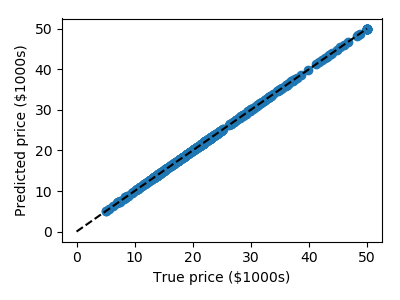
3.6.9.1. Measuring Decision Tree performance

Demonstrates overfit when testing on train set.

Get the data

 
   from sklearn.datasets import load_boston
data = load_boston()

Train and test a model

 
   from sklearn.tree import DecisionTreeRegressor
clf = DecisionTreeRegressor().fit(data.data, data.target)

predicted = clf.predict(data.data)
expected = data.target

Plot predicted as a function of expected

 
   from matplotlib import pyplot as plt
plt.figure(figsize=(4, 3))
plt.scatter(expected, predicted)
plt.plot([0, 50], [0, 50], '--k')
plt.axis('tight')
plt.xlabel('True price ($1000s)')
plt.ylabel('Predicted price ($1000s)')
plt.tight_layout()
 
  

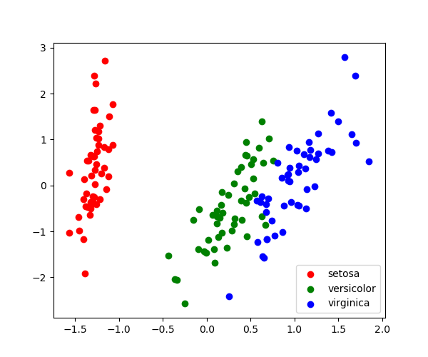
../../../_images/sphx_glr_plot_measuring_performance_001.png

3.6.9.2. Demo PCA in 2D

Load the iris data

 
   from sklearn import datasets
iris = datasets.load_iris()
X = iris.data
y = iris.target

Fit a PCA

 
   from sklearn.decomposition import PCA
pca = PCA(n_components=2, whiten=True)
pca.fit(X)

Project the data in 2D

 
   X_pca = pca.transform(X)

Visualize the data

 
   target_ids = range(len(iris.target_names))

from matplotlib import pyplot as plt
plt.figure(figsize=(6, 5))
for i, c, label in zip(target_ids, 'rgbcmykw', iris.target_names):
    plt.scatter(X_pca[y == i, 0], X_pca[y == i, 1],
               c=c, label=label)
plt.legend()
plt.show()
 
  

../../../_images/sphx_glr_plot_pca_001.png

3.6.9.3. A simple linear regression

 
   import numpy as np
import matplotlib.pyplot as plt
from sklearn.linear_model import LinearRegression

# x from 0 to 30
x = 30 * np.random.random((20, 1))

# y = a*x + b with noise
y = 0.5 * x + 1.0 + np.random.normal(size=x.shape)

# create a linear regression model
model = LinearRegression()
model.fit(x, y)

# predict y from the data
x_new = np.linspace(0, 30, 100)
y_new = model.predict(x_new[:, np.newaxis])

# plot the results
plt.figure(figsize=(4, 3))
ax = plt.axes()
ax.scatter(x, y)
ax.plot(x_new, y_new)

ax.set_xlabel('x')
ax.set_ylabel('y')

ax.axis('tight')


plt.show() 
  

3.6.9.4. Plot 2D views of the iris dataset

Plot a simple scatter plot of 2 features of the iris dataset.

Note that more elaborate visualization of this dataset is detailed in theStatistics in Python chapter.

 
   # Load the data
from sklearn.datasets import load_iris
iris = load_iris()

from matplotlib import pyplot as plt

# The indices of the features that we are plotting
x_index = 0
y_index = 1

# this formatter will label the colorbar with the correct target names
formatter = plt.FuncFormatter(lambda i, *args: iris.target_names[int(i)])

plt.figure(figsize=(5, 4))
plt.scatter(iris.data[:, x_index], iris.data[:, y_index], c=iris.target)
plt.colorbar(ticks=[0, 1, 2], format=formatter)
plt.xlabel(iris.feature_names[x_index])
plt.ylabel(iris.feature_names[y_index])

plt.tight_layout()
plt.show() 
  

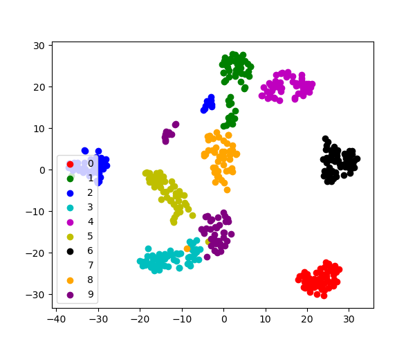
3.6.9.5. tSNE to visualize digits

Here we use sklearn.manifold.TSNE to visualize the digits datasets. Indeed, the digits are vectors in a 8*8 = 64 dimensional space. We want to project them in 2D for visualization. tSNE is often a good solution, as it groups and separates data points based on their local relationship.

Load the iris data

 
   from sklearn import datasets
digits = datasets.load_digits()
# Take the first 500 data points: it's hard to see 1500 points
X = digits.data[:500]
y = digits.target[:500]
 
  

Fit and transform with a TSNE

 
   from sklearn.manifold import TSNE
tsne = TSNE(n_components=2, random_state=0)

Project the data in 2D

 
   X_2d = tsne.fit_transform(X)

Visualize the data

 
   target_ids = range(len(digits.target_names))

from matplotlib import pyplot as plt
plt.figure(figsize=(6, 5))
colors = 'r', 'g', 'b', 'c', 'm', 'y', 'k', 'w', 'orange', 'purple'
for i, c, label in zip(target_ids, colors, digits.target_names):
    plt.scatter(X_2d[y == i, 0], X_2d[y == i, 1], c=c, label=label)
plt.legend()
plt.show()
 
  

../../../_images/sphx_glr_plot_tsne_001.png

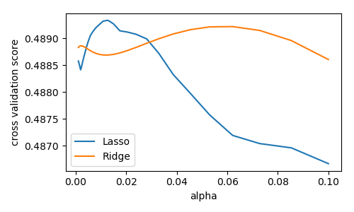
3.6.9.6. Use the RidgeCV and LassoCV to set the regularization parameter

Load the diabetes dataset

 
   from sklearn.datasets import load_diabetes
data = load_diabetes()
X, y = data.data, data.target
print(X.shape)

Out:

 
   (442, 10)

Compute the cross-validation score with the default hyper-parameters

 
   from sklearn.model_selection import cross_val_score
from sklearn.linear_model import Ridge, Lasso

for Model in [Ridge, Lasso]:
    model = Model()
    print('%s: %s' % (Model.__name__,
                      cross_val_score(model, X, y).mean()))
 
  

Out:

 
   Ridge: 0.409427438303
Lasso: 0.353800083299

We compute the cross-validation score as a function of alpha, the strength of the regularization for Lasso and Ridge

 
   import numpy as np
from matplotlib import pyplot as plt

alphas = np.logspace(-3, -1, 30)

plt.figure(figsize=(5, 3))

for Model in [Lasso, Ridge]:
    scores = [cross_val_score(Model(alpha), X, y, cv=3).mean()
            for alpha in alphas]
    plt.plot(alphas, scores, label=Model.__name__)

plt.legend(loc='lower left')
plt.xlabel('alpha')
plt.ylabel('cross validation score')
plt.tight_layout()
plt.show()
 
  

../../../_images/sphx_glr_plot_linear_model_cv_001.png

3.6.9.7. Plot variance and regularization in linear models

 
   import numpy as np

# Smaller figures
from matplotlib import pyplot as plt
plt.rcParams['figure.figsize'] = (3, 2)

We consider the situation where we have only 2 data point

 
   X = np.c_[ .5, 1].T
y = [.5, 1]
X_test = np.c_[ 0, 2].T

Without noise, as linear regression fits the data perfectly

 
   from sklearn import linear_model
regr = linear_model.LinearRegression()
regr.fit(X, y)
plt.plot(X, y, 'o')
plt.plot(X_test, regr.predict(X_test))
 
  

../../../_images/sphx_glr_plot_variance_linear_regr_001.png

In real life situation, we have noise (e.g. measurement noise) in our data:

 
   np.random.seed(0)
for _ in range(6):
    noisy_X = X + np.random.normal(loc=0, scale=.1, size=X.shape)
    plt.plot(noisy_X, y, 'o')
    regr.fit(noisy_X, y)
    plt.plot(X_test, regr.predict(X_test))
 
  

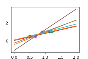
../../../_images/sphx_glr_plot_variance_linear_regr_002.png

As we can see, our linear model captures and amplifies the noise in the data. It displays a lot of variance.

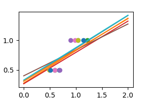
We can use another linear estimator that uses regularization, the Ridgeestimator. This estimator regularizes the coefficients by shrinking them to zero, under the assumption that very high correlations are often spurious. The alpha parameter controls the amount of shrinkage used.

 
   regr = linear_model.Ridge(alpha=.1)
np.random.seed(0)
for _ in range(6):
    noisy_X = X + np.random.normal(loc=0, scale=.1, size=X.shape)
    plt.plot(noisy_X, y, 'o')
    regr.fit(noisy_X, y)
    plt.plot(X_test, regr.predict(X_test))

plt.show()
 
  

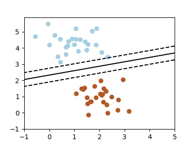
../../../_images/sphx_glr_plot_variance_linear_regr_003.png

3.6.9.8. Simple picture of the formal problem of machine learning

This example generates simple synthetic data ploints and shows a separating hyperplane on them.

 
   import numpy as np
import matplotlib.pyplot as plt
from sklearn.linear_model import SGDClassifier
from sklearn.datasets.samples_generator import make_blobs

# we create 50 separable synthetic points
X, Y = make_blobs(n_samples=50, centers=2,
                  random_state=0, cluster_std=0.60)

# fit the model
clf = SGDClassifier(loss="hinge", alpha=0.01,
                    n_iter=200, fit_intercept=True)
clf.fit(X, Y)

# plot the line, the points, and the nearest vectors to the plane
xx = np.linspace(-1, 5, 10)
yy = np.linspace(-1, 5, 10)

X1, X2 = np.meshgrid(xx, yy)
Z = np.empty(X1.shape)
for (i, j), val in np.ndenumerate(X1):
    x1 = val
    x2 = X2[i, j]
    p = clf.decision_function([[x1, x2]])
    Z[i, j] = p[0]

plt.figure(figsize=(4, 3))
ax = plt.axes()
ax.contour(X1, X2, Z, [-1.0, 0.0, 1.0], colors='k',
           linestyles=['dashed', 'solid', 'dashed'])
ax.scatter(X[:, 0], X[:, 1], c=Y, cmap=plt.cm.Paired)

ax.axis('tight')


plt.show() 
  

3.6.9.9. Compare classifiers on the digits data

Compare the performance of a variety of classifiers on a test set for the digits data.

Out:

 
   LinearSVC: 0.927190026916
GaussianNB: 0.833274168101
KNeighborsClassifier: 0.980456280495
------------------
LinearSVC(loss='l1'): 0.9325901988044822
LinearSVC(loss='l2'): 0.9165874249889226
-------------------
KNeighbors(n_neighbors=1): 0.9913675218842191
KNeighbors(n_neighbors=2): 0.9848442068835102
KNeighbors(n_neighbors=3): 0.9867753449543099
KNeighbors(n_neighbors=4): 0.9803719053818863
KNeighbors(n_neighbors=5): 0.9804562804949924
KNeighbors(n_neighbors=6): 0.9757924194139573
KNeighbors(n_neighbors=7): 0.9780645792142071
KNeighbors(n_neighbors=8): 0.9780645792142071
KNeighbors(n_neighbors=9): 0.9780645792142071
KNeighbors(n_neighbors=10): 0.9755550897728812
 
  

 
   from sklearn import model_selection, datasets, metrics
from sklearn.svm import LinearSVC
from sklearn.naive_bayes import GaussianNB
from sklearn.neighbors import KNeighborsClassifier

digits = datasets.load_digits()
X = digits.data
y = digits.target
X_train, X_test, y_train, y_test = model_selection.train_test_split(X, y,
                            test_size=0.25, random_state=0)

for Model in [LinearSVC, GaussianNB, KNeighborsClassifier]:
    clf = Model().fit(X_train, y_train)
    y_pred = clf.predict(X_test)
    print('%s: %s' %
          (Model.__name__, metrics.f1_score(y_test, y_pred, average="macro")))

print('------------------')

# test SVC loss
for loss in ['l1', 'l2']:
    clf = LinearSVC(loss=loss).fit(X_train, y_train)
    y_pred = clf.predict(X_test)
    print("LinearSVC(loss='{0}'): {1}".format(loss,
          metrics.f1_score(y_test, y_pred, average="macro")))

print('-------------------')

# test the number of neighbors
for n_neighbors in range(1, 11):
    clf = KNeighborsClassifier(n_neighbors=n_neighbors).fit(X_train, y_train)
    y_pred = clf.predict(X_test)
    print("KNeighbors(n_neighbors={0}): {1}".format(n_neighbors,
        metrics.f1_score(y_test, y_pred, average="macro"))) 
  

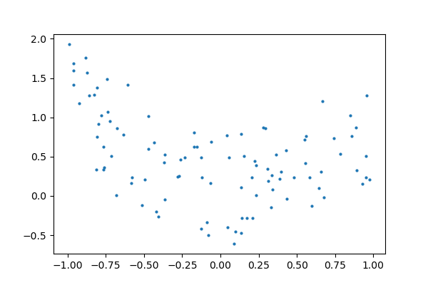
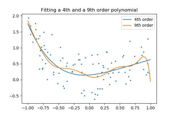
3.6.9.10. Plot fitting a 9th order polynomial

Fits data generated from a 9th order polynomial with model of 4th order and 9th order polynomials, to demonstrate that often simpler models are to be prefered

 
   import numpy as np
from matplotlib import pyplot as plt
from matplotlib.colors import ListedColormap

from sklearn import linear_model

# Create color maps for 3-class classification problem, as with iris
cmap_light = ListedColormap(['#FFAAAA', '#AAFFAA', '#AAAAFF'])
cmap_bold = ListedColormap(['#FF0000', '#00FF00', '#0000FF'])

rng = np.random.RandomState(0)
x = 2*rng.rand(100) - 1

f = lambda t: 1.2 * t**2 + .1 * t**3 - .4 * t **5 - .5 * t ** 9
y = f(x) + .4 * rng.normal(size=100)

x_test = np.linspace(-1, 1, 100)

The data

 
   plt.figure(figsize=(6, 4))
plt.scatter(x, y, s=4)

../../../_images/sphx_glr_plot_polynomial_regression_001.png

Fitting 4th and 9th order polynomials

For this we need to engineer features: the n_th powers of x:

 
   plt.figure(figsize=(6, 4))
plt.scatter(x, y, s=4)

X = np.array([x**i for i in range(5)]).T
X_test = np.array([x_test**i for i in range(5)]).T
regr = linear_model.LinearRegression()
regr.fit(X, y)
plt.plot(x_test, regr.predict(X_test), label='4th order')

X = np.array([x**i for i in range(10)]).T
X_test = np.array([x_test**i for i in range(10)]).T
regr = linear_model.LinearRegression()
regr.fit(X, y)
plt.plot(x_test, regr.predict(X_test), label='9th order')

plt.legend(loc='best')
plt.axis('tight')
plt.title('Fitting a 4th and a 9th order polynomial')
 
  

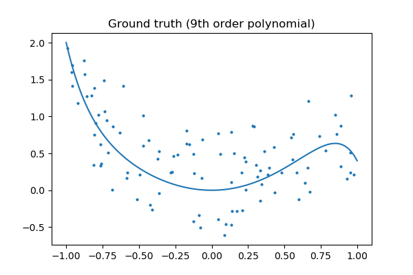
../../../_images/sphx_glr_plot_polynomial_regression_002.png

Ground truth

 
   plt.figure(figsize=(6, 4))
plt.scatter(x, y, s=4)
plt.plot(x_test, f(x_test), label="truth")
plt.axis('tight')
plt.title('Ground truth (9th order polynomial)')

plt.show()
 
  

../../../_images/sphx_glr_plot_polynomial_regression_003.png

3.6.9.11. A simple regression analysis on the Boston housing data

Here we perform a simple regression analysis on the Boston housing data, exploring two types of regressors.

 
   from sklearn.datasets import load_boston
data = load_boston()

Print a histogram of the quantity to predict: price

 
   import matplotlib.pyplot as plt
plt.figure(figsize=(4, 3))
plt.hist(data.target)
plt.xlabel('price ($1000s)')
plt.ylabel('count')
plt.tight_layout()
 
  

Print the join histogram for each feature

 
   for index, feature_name in enumerate(data.feature_names):
    plt.figure(figsize=(4, 3))
    plt.scatter(data.data[:, index], data.target)
    plt.ylabel('Price', size=15)
    plt.xlabel(feature_name, size=15)
    plt.tight_layout()
 
  

Simple prediction

 
   from sklearn.model_selection import train_test_split
X_train, X_test, y_train, y_test = train_test_split(data.data, data.target)

from sklearn.linear_model import LinearRegression
clf = LinearRegression()
clf.fit(X_train, y_train)
predicted = clf.predict(X_test)
expected = y_test

plt.figure(figsize=(4, 3))
plt.scatter(expected, predicted)
plt.plot([0, 50], [0, 50], '--k')
plt.axis('tight')
plt.xlabel('True price ($1000s)')
plt.ylabel('Predicted price ($1000s)')
plt.tight_layout()
 
  

../../../_images/sphx_glr_plot_boston_prediction_015.png

Prediction with gradient boosted tree

 
   from sklearn.ensemble import GradientBoostingRegressor

clf = GradientBoostingRegressor()
clf.fit(X_train, y_train)

predicted = clf.predict(X_test)
expected = y_test

plt.figure(figsize=(4, 3))
plt.scatter(expected, predicted)
plt.plot([0, 50], [0, 50], '--k')
plt.axis('tight')
plt.xlabel('True price ($1000s)')
plt.ylabel('Predicted price ($1000s)')
plt.tight_layout()
 
  

../../../_images/sphx_glr_plot_boston_prediction_016.png

Print the error rate

 
   import numpy as np
print("RMS: %r " % np.sqrt(np.mean((predicted - expected) ** 2)))

plt.show()

Out:

 
   RMS: 3.3940265988986305 
  

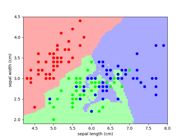
3.6.9.12. Nearest-neighbor prediction on iris

Plot the decision boundary of nearest neighbor decision on iris, first with a single nearest neighbor, and then using 3 nearest neighbors.

 
   import numpy as np
from matplotlib import pyplot as plt
from sklearn import neighbors, datasets
from matplotlib.colors import ListedColormap

# Create color maps for 3-class classification problem, as with iris
cmap_light = ListedColormap(['#FFAAAA', '#AAFFAA', '#AAAAFF'])
cmap_bold = ListedColormap(['#FF0000', '#00FF00', '#0000FF'])

iris = datasets.load_iris()
X = iris.data[:, :2]  # we only take the first two features. We could
                    # avoid this ugly slicing by using a two-dim dataset
y = iris.target

knn = neighbors.KNeighborsClassifier(n_neighbors=1)
knn.fit(X, y)

x_min, x_max = X[:, 0].min() - .1, X[:, 0].max() + .1
y_min, y_max = X[:, 1].min() - .1, X[:, 1].max() + .1
xx, yy = np.meshgrid(np.linspace(x_min, x_max, 100),
                        np.linspace(y_min, y_max, 100))
Z = knn.predict(np.c_[xx.ravel(), yy.ravel()])
 
  

Put the result into a color plot

 
   Z = Z.reshape(xx.shape)
plt.figure()
plt.pcolormesh(xx, yy, Z, cmap=cmap_light)

# Plot also the training points
plt.scatter(X[:, 0], X[:, 1], c=y, cmap=cmap_bold)
plt.xlabel('sepal length (cm)')
plt.ylabel('sepal width (cm)')
plt.axis('tight')
 
  

And now, redo the analysis with 3 neighbors

 
   knn = neighbors.KNeighborsClassifier(n_neighbors=3)
knn.fit(X, y)

Z = knn.predict(np.c_[xx.ravel(), yy.ravel()])

# Put the result into a color plot
Z = Z.reshape(xx.shape)
plt.figure()
plt.pcolormesh(xx, yy, Z, cmap=cmap_light)

# Plot also the training points
plt.scatter(X[:, 0], X[:, 1], c=y, cmap=cmap_bold)
plt.xlabel('sepal length (cm)')
plt.ylabel('sepal width (cm)')
plt.axis('tight')

plt.show()
 
  

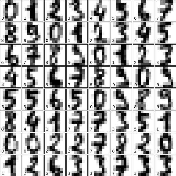
../../../_images/sphx_glr_plot_iris_knn_002.png

3.6.9.13. Simple visualization and classification of the digits dataset

Plot the first few samples of the digits dataset and a 2D representation built using PCA, then do a simple classification

 
   from sklearn.datasets import load_digits
digits = load_digits()

Plot the data: images of digits

Each data in a 8x8 image

 
    from matplotlib import pyplot as plt
fig = plt.figure(figsize=(6, 6))  # figure size in inches
fig.subplots_adjust(left=0, right=1, bottom=0, top=1, hspace=0.05, wspace=0.05)

for i in range(64):
    ax = fig.add_subplot(8, 8, i + 1, xticks=[], yticks=[])
    ax.imshow(digits.images[i], cmap=plt.cm.binary, interpolation='nearest')
    # label the image with the target value
    ax.text(0, 7, str(digits.target[i]))
 
   

../../../_images/sphx_glr_plot_digits_simple_classif_001.png

Plot a projection on the 2 first principal axis

 
    plt.figure()

from sklearn.decomposition import PCA
pca = PCA(n_components=2)
proj = pca.fit_transform(digits.data)
plt.scatter(proj[:, 0], proj[:, 1], c=digits.target)
plt.colorbar()
 
   

../../../_images/sphx_glr_plot_digits_simple_classif_002.png

Classify with Gaussian naive Bayes

 
    from sklearn.naive_bayes import GaussianNB
from sklearn.model_selection import train_test_split

# split the data into training and validation sets
X_train, X_test, y_train, y_test = train_test_split(digits.data, digits.target)

# train the model
clf = GaussianNB()
clf.fit(X_train, y_train)

# use the model to predict the labels of the test data
predicted = clf.predict(X_test)
expected = y_test

# Plot the prediction
fig = plt.figure(figsize=(6, 6))  # figure size in inches
fig.subplots_adjust(left=0, right=1, bottom=0, top=1, hspace=0.05, wspace=0.05)

# plot the digits: each image is 8x8 pixels
for i in range(64):
    ax = fig.add_subplot(8, 8, i + 1, xticks=[], yticks=[])
    ax.imshow(X_test.reshape(-1, 8, 8)[i], cmap=plt.cm.binary,
              interpolation='nearest')

    # label the image with the target value
    if predicted[i] == expected[i]:
        ax.text(0, 7, str(predicted[i]), color='green')
    else:
        ax.text(0, 7, str(predicted[i]), color='red')
 
   

../../../_images/sphx_glr_plot_digits_simple_classif_003.png

Quantify the performance

First print the number of correct matches

 
    matches = (predicted == expected)
print(matches.sum())

Out:

The total number of data points

 
    print(len(matches))

Out:

And now, the ration of correct predictions

 
    matches.sum() / float(len(matches))

Print the classification report

 
    from sklearn import metrics
print(metrics.classification_report(expected, predicted))

Out:

 
    precision    recall  f1-score   support

          0       1.00      0.93      0.96        40
          1       0.82      0.85      0.84        48
          2       0.91      0.69      0.78        45
          3       0.96      0.83      0.89        58
          4       0.91      0.89      0.90        36
          5       0.91      0.85      0.88        48
          6       0.93      0.98      0.95        43
          7       0.75      0.98      0.85        47
          8       0.59      0.81      0.68        42
          9       0.91      0.74      0.82        43

avg / total       0.87      0.85      0.86       450
 
   

Print the confusion matrix

 
    print(metrics.confusion_matrix(expected, predicted))

plt.show()

Out:

 
    [[37  0  0  0  2  0  0  1  0  0]
 [ 0 41  0  0  0  0  1  0  4  2]
 [ 0  2 31  0  0  0  1  0 11  0]
 [ 0  0  2 48  0  1  0  2  4  1]
 [ 0  1  1  0 32  0  0  1  1  0]
 [ 0  1  0  1  1 41  0  4  0  0]
 [ 0  0  0  0  0  1 42  0  0  0]
 [ 0  0  0  0  0  1  0 46  0  0]
 [ 0  4  0  0  0  1  0  3 34  0]
 [ 0  1  0  1  0  0  1  4  4 32]] 
   

3.6.9.14. The eigenfaces example: chaining PCA and SVMs

The goal of this example is to show how an unsupervised method and a supervised one can be chained for better prediction. It starts with a didactic but lengthy way of doing things, and finishes with the idiomatic approach to pipelining in scikit-learn.

Here we’ll take a look at a simple facial recognition example. Ideally, we would use a dataset consisting of a subset of the Labeled Faces in the Wilddata that is available with sklearn.datasets.fetch_lfw_people(). However, this is a relatively large download (~200MB) so we will do the tutorial on a simpler, less rich dataset. Feel free to explore the LFW dataset.

 
   from sklearn import datasets
faces = datasets.fetch_olivetti_faces()
faces.data.shape

Let’s visualize these faces to see what we’re working with

 
   from matplotlib import pyplot as plt
fig = plt.figure(figsize=(8, 6))
# plot several images
for i in range(15):
    ax = fig.add_subplot(3, 5, i + 1, xticks=[], yticks=[])
    ax.imshow(faces.images[i], cmap=plt.cm.bone)
 
  

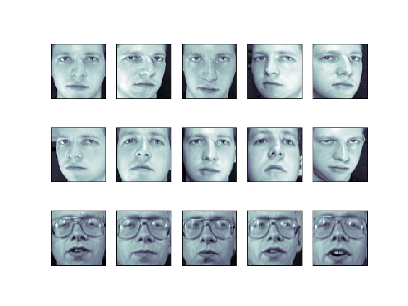
../../../_images/sphx_glr_plot_eigenfaces_001.png

Note is that these faces have already been localized and scaled to a common size. This is an important preprocessing piece for facial recognition, and is a process that can require a large collection of training data. This can be done in scikit-learn, but the challenge is gathering a sufficient amount of training data for the algorithm to work. Fortunately, this piece is common enough that it has been done. One good resource is OpenCV, the Open Computer Vision Library.

We’ll perform a Support Vector classification of the images. We’ll do a typical train-test split on the images:

 
   from sklearn.model_selection import train_test_split
X_train, X_test, y_train, y_test = train_test_split(faces.data,
        faces.target, random_state=0)

print(X_train.shape, X_test.shape)

Out:

 
   (300, 4096) (100, 4096)

Preprocessing: Principal Component Analysis

1850 dimensions is a lot for SVM. We can use PCA to reduce these 1850 features to a manageable size, while maintaining most of the information in the dataset.

 
    from sklearn import decomposition
pca = decomposition.PCA(n_components=150, whiten=True)
pca.fit(X_train)

One interesting part of PCA is that it computes the “mean” face, which can be interesting to examine:

 
    plt.imshow(pca.mean_.reshape(faces.images[0].shape),
           cmap=plt.cm.bone)

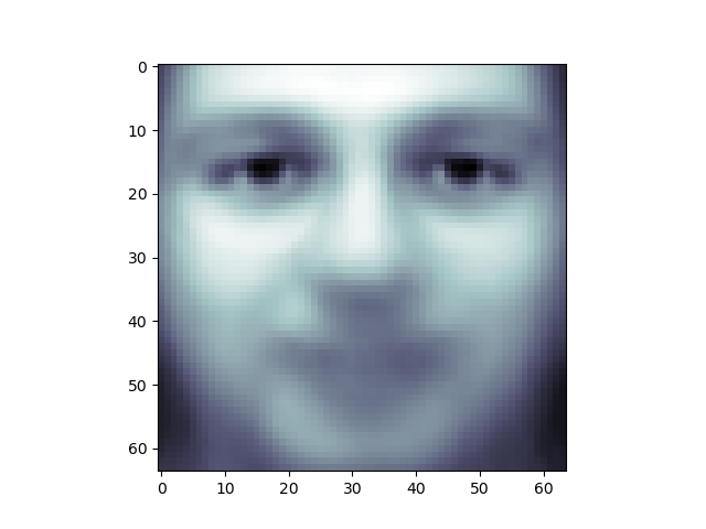
../../../_images/sphx_glr_plot_eigenfaces_002.png

The principal components measure deviations about this mean along orthogonal axes.

 
    print(pca.components_.shape)

Out:

 
    (150, 4096)

It is also interesting to visualize these principal components:

 
    fig = plt.figure(figsize=(16, 6))
for i in range(30):
    ax = fig.add_subplot(3, 10, i + 1, xticks=[], yticks=[])
    ax.imshow(pca.components_[i].reshape(faces.images[0].shape),
              cmap=plt.cm.bone)
 
   

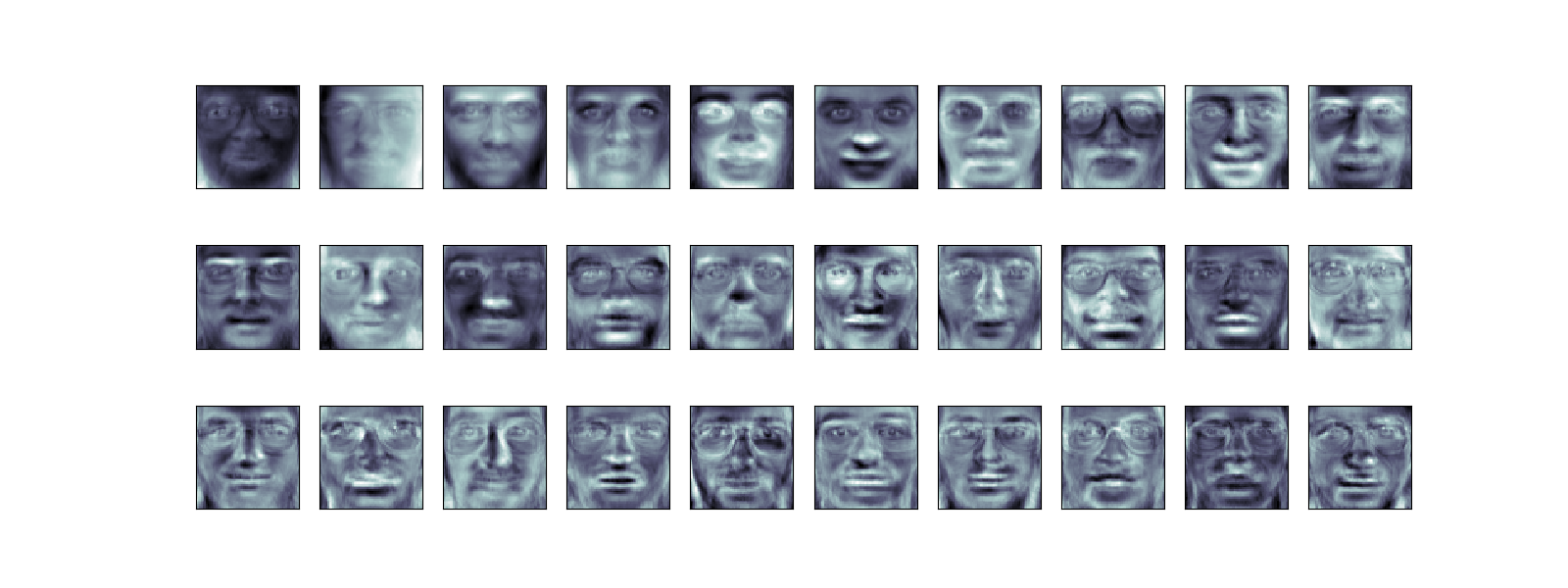
../../../_images/sphx_glr_plot_eigenfaces_003.png

The components (“eigenfaces”) are ordered by their importance from top-left to bottom-right. We see that the first few components seem to primarily take care of lighting conditions; the remaining components pull out certain identifying features: the nose, eyes, eyebrows, etc.

With this projection computed, we can now project our original training and test data onto the PCA basis:

 
    X_train_pca = pca.transform(X_train)
X_test_pca = pca.transform(X_test)
print(X_train_pca.shape)

Out:

 
    (300, 150)

 
    print(X_test_pca.shape)

Out:

 
    (100, 150)

These projected components correspond to factors in a linear combination of component images such that the combination approaches the original face.

Doing the Learning: Support Vector Machines

Now we’ll perform support-vector-machine classification on this reduced dataset:

 
    from sklearn import svm
clf = svm.SVC(C=5., gamma=0.001)
clf.fit(X_train_pca, y_train)

Finally, we can evaluate how well this classification did. First, we might plot a few of the test-cases with the labels learned from the training set:

 
    import numpy as np
fig = plt.figure(figsize=(8, 6))
for i in range(15):
    ax = fig.add_subplot(3, 5, i + 1, xticks=[], yticks=[])
    ax.imshow(X_test[i].reshape(faces.images[0].shape),
              cmap=plt.cm.bone)
    y_pred = clf.predict(X_test_pca[i, np.newaxis])[0]
    color = ('black' if y_pred == y_test[i] else 'red')
    ax.set_title(faces.target[y_pred],
                 fontsize='small', color=color)
 
   

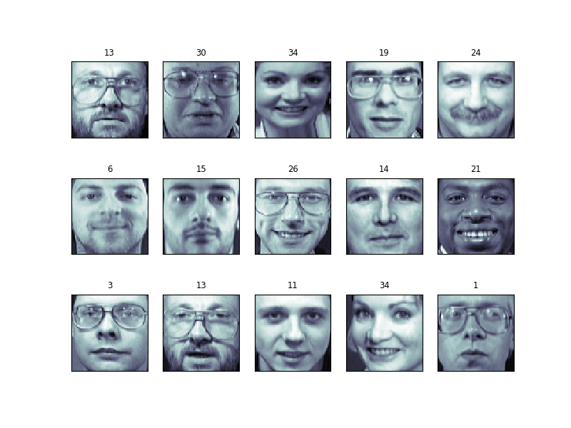
../../../_images/sphx_glr_plot_eigenfaces_004.png

The classifier is correct on an impressive number of images given the simplicity of its learning model! Using a linear classifier on 150 features derived from the pixel-level data, the algorithm correctly identifies a large number of the people in the images.

Again, we can quantify this effectiveness using one of several measures fromsklearn.metrics. First we can do the classification report, which shows the precision, recall and other measures of the “goodness” of the classification:

 
    from sklearn import metrics
y_pred = clf.predict(X_test_pca)
print(metrics.classification_report(y_test, y_pred))

Out:

 
    precision    recall  f1-score   support

          0       1.00      0.67      0.80         6
          1       1.00      1.00      1.00         4
          2       0.50      1.00      0.67         2
          3       1.00      1.00      1.00         1
          4       1.00      1.00      1.00         1
          5       1.00      1.00      1.00         5
          6       1.00      1.00      1.00         4
          7       1.00      0.67      0.80         3
          9       1.00      1.00      1.00         1
         10       1.00      1.00      1.00         4
         11       1.00      1.00      1.00         1
         12       0.67      1.00      0.80         2
         13       1.00      1.00      1.00         3
         14       1.00      1.00      1.00         5
         15       1.00      1.00      1.00         3
         17       1.00      1.00      1.00         6
         19       1.00      1.00      1.00         4
         20       1.00      1.00      1.00         1
         21       1.00      1.00      1.00         1
         22       1.00      1.00      1.00         2
         23       0.50      1.00      0.67         1
         24       1.00      1.00      1.00         2
         25       1.00      0.50      0.67         2
         26       1.00      0.75      0.86         4
         27       1.00      1.00      1.00         1
         28       0.67      1.00      0.80         2
         29       1.00      1.00      1.00         3
         30       1.00      1.00      1.00         4
         31       1.00      1.00      1.00         3
         32       1.00      1.00      1.00         3
         33       1.00      1.00      1.00         2
         34       1.00      1.00      1.00         3
         35       1.00      1.00      1.00         1
         36       1.00      1.00      1.00         3
         37       1.00      1.00      1.00         3
         38       1.00      1.00      1.00         1
         39       1.00      1.00      1.00         3

avg / total       0.97      0.95      0.95       100
 
   

Another interesting metric is the confusion matrix, which indicates how often any two items are mixed-up. The confusion matrix of a perfect classifier would only have nonzero entries on the diagonal, with zeros on the off-diagonal:

 
    print(metrics.confusion_matrix(y_test, y_pred))

Out:

 
    [[4 0 0 ..., 0 0 0]
 [0 4 0 ..., 0 0 0]
 [0 0 2 ..., 0 0 0]
 ...,
 [0 0 0 ..., 3 0 0]
 [0 0 0 ..., 0 1 0]
 [0 0 0 ..., 0 0 3]]
 
   

Pipelining

Above we used PCA as a pre-processing step before applying our support vector machine classifier. Plugging the output of one estimator directly into the input of a second estimator is a commonly used pattern; for this reason scikit-learn provides a Pipeline object which automates this process. The above problem can be re-expressed as a pipeline as follows:

 
    from sklearn.pipeline import Pipeline
clf = Pipeline([('pca', decomposition.PCA(n_components=150, whiten=True)),
                ('svm', svm.LinearSVC(C=1.0))])

clf.fit(X_train, y_train)

y_pred = clf.predict(X_test)
print(metrics.confusion_matrix(y_pred, y_test))
plt.show()

Out:

 
    [[5 0 0 ..., 0 0 0]
 [0 4 0 ..., 0 0 0]
 [0 0 1 ..., 0 0 0]
 ...,
 [0 0 0 ..., 3 0 0]
 [0 0 0 ..., 0 1 0]
 [0 0 0 ..., 0 0 3]]
 
   

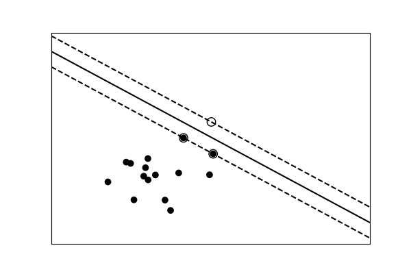
3.6.9.15. Example of linear and non-linear models

This is an example plot from the tutorial which accompanies an explanation of the support vector machine GUI.

 
   import numpy as np
from matplotlib import pyplot as plt

from sklearn import svm

data that is linearly separable

 
   def linear_model(rseed=42, n_samples=30):
    " Generate data according to a linear model"
    np.random.seed(rseed)

    data = np.random.normal(0, 10, (n_samples, 2))
    data[:n_samples // 2] -= 15
    data[n_samples // 2:] += 15

    labels = np.ones(n_samples)
    labels[:n_samples // 2] = -1

    return data, labels


X, y = linear_model()
clf = svm.SVC(kernel='linear')
clf.fit(X, y)

plt.figure(figsize=(6, 4))
ax = plt.subplot(111, xticks=[], yticks=[])
ax.scatter(X[:, 0], X[:, 1], c=y, cmap=plt.cm.bone)

ax.scatter(clf.support_vectors_[:, 0],
            clf.support_vectors_[:, 1],
            s=80, edgecolors="k", facecolors="none")

delta = 1
y_min, y_max = -50, 50
x_min, x_max = -50, 50
x = np.arange(x_min, x_max + delta, delta)
y = np.arange(y_min, y_max + delta, delta)
X1, X2 = np.meshgrid(x, y)
Z = clf.decision_function(np.c_[X1.ravel(), X2.ravel()])
Z = Z.reshape(X1.shape)

ax.contour(X1, X2, Z, [-1.0, 0.0, 1.0], colors='k',
           linestyles=['dashed', 'solid', 'dashed'])
 
  

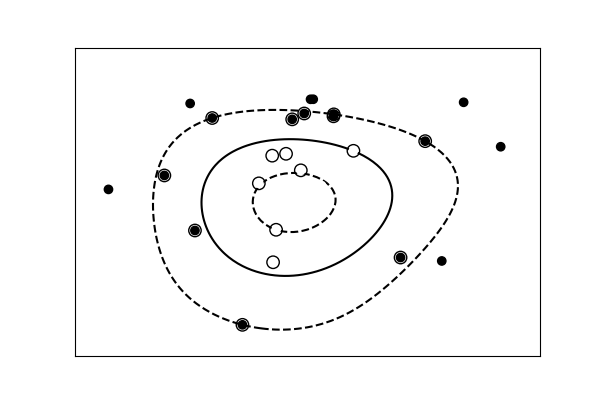
../../../_images/sphx_glr_plot_svm_non_linear_001.png

data with a non-linear separation

 
   def nonlinear_model(rseed=42, n_samples=30):
    radius = 40 * np.random.random(n_samples)
    far_pts = radius > 20
    radius[far_pts] *= 1.2
    radius[~far_pts] *= 1.1

    theta = np.random.random(n_samples) * np.pi * 2

    data = np.empty((n_samples, 2))
    data[:, 0] = radius * np.cos(theta)
    data[:, 1] = radius * np.sin(theta)

    labels = np.ones(n_samples)
    labels[far_pts] = -1

    return data, labels


X, y = nonlinear_model()
clf = svm.SVC(kernel='rbf', gamma=0.001, coef0=0, degree=3)
clf.fit(X, y)

plt.figure(figsize=(6, 4))
ax = plt.subplot(1, 1, 1, xticks=[], yticks=[])
ax.scatter(X[:, 0], X[:, 1], c=y, cmap=plt.cm.bone, zorder=2)

ax.scatter(clf.support_vectors_[:, 0], clf.support_vectors_[:, 1],
           s=80, edgecolors="k", facecolors="none")

delta = 1
y_min, y_max = -50, 50
x_min, x_max = -50, 50
x = np.arange(x_min, x_max + delta, delta)
y = np.arange(y_min, y_max + delta, delta)
X1, X2 = np.meshgrid(x, y)
Z = clf.decision_function(np.c_[X1.ravel(), X2.ravel()])
Z = Z.reshape(X1.shape)

ax.contour(X1, X2, Z, [-1.0, 0.0, 1.0], colors='k',
            linestyles=['dashed', 'solid', 'dashed'], zorder=1)

plt.show()
 
  

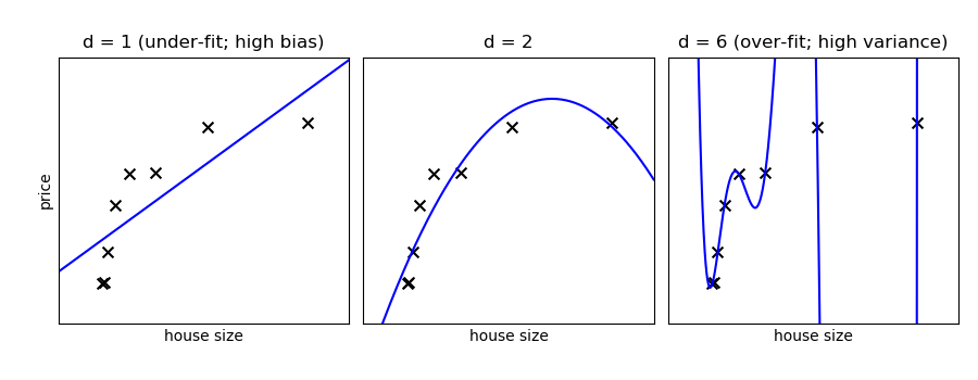
../../../_images/sphx_glr_plot_svm_non_linear_002.png

3.6.9.16. Bias and variance of polynomial fit

Demo overfitting, underfitting, and validation and learning curves with polynomial regression.

Fit polynomes of different degrees to a dataset: for too small a degree, the model underfits, while for too large a degree, it overfits.

 
   import numpy as np
import matplotlib.pyplot as plt

def generating_func(x, err=0.5):
    return np.random.normal(10 - 1. / (x + 0.1), err)

A polynomial regression

 
   from sklearn.pipeline import make_pipeline
from sklearn.linear_model import LinearRegression
from sklearn.preprocessing import PolynomialFeatures

A simple figure to illustrate the problem

 
   n_samples = 8

np.random.seed(0)
x = 10 ** np.linspace(-2, 0, n_samples)
y = generating_func(x)

x_test = np.linspace(-0.2, 1.2, 1000)

titles = ['d = 1 (under-fit; high bias)',
          'd = 2',
          'd = 6 (over-fit; high variance)']
degrees = [1, 2, 6]

fig = plt.figure(figsize=(9, 3.5))
fig.subplots_adjust(left=0.06, right=0.98, bottom=0.15, top=0.85, wspace=0.05)

for i, d in enumerate(degrees):
    ax = fig.add_subplot(131 + i, xticks=[], yticks=[])
    ax.scatter(x, y, marker='x', c='k', s=50)

    model = make_pipeline(PolynomialFeatures(d), LinearRegression())
    model.fit(x[:, np.newaxis], y)
    ax.plot(x_test, model.predict(x_test[:, np.newaxis]), '-b')

    ax.set_xlim(-0.2, 1.2)
    ax.set_ylim(0, 12)
    ax.set_xlabel('house size')
    if i == 0:
        ax.set_ylabel('price')

    ax.set_title(titles[i])
 
  

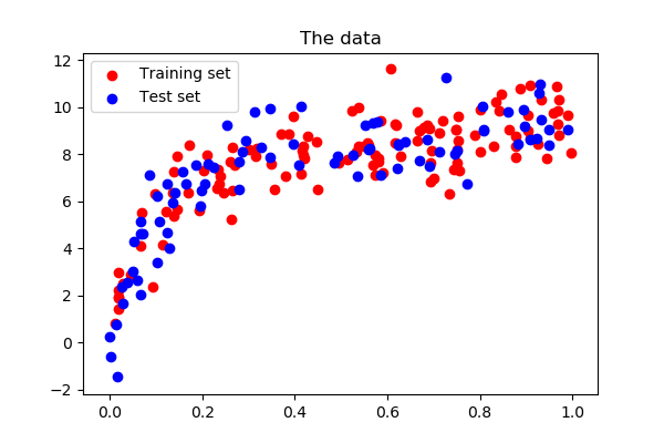
../../../_images/sphx_glr_plot_bias_variance_001.png

Generate a larger dataset

 
   from sklearn.model_selection import train_test_split

n_samples = 200
test_size = 0.4
error = 1.0

# randomly sample the data
np.random.seed(1)
x = np.random.random(n_samples)
y = generating_func(x, error)

# split into training, validation, and testing sets.
x_train, x_test, y_train, y_test = train_test_split(x, y, test_size=test_size)

# show the training and validation sets
plt.figure(figsize=(6, 4))
plt.scatter(x_train, y_train, color='red', label='Training set')
plt.scatter(x_test, y_test, color='blue', label='Test set')
plt.title('The data')
plt.legend(loc='best')
 
  

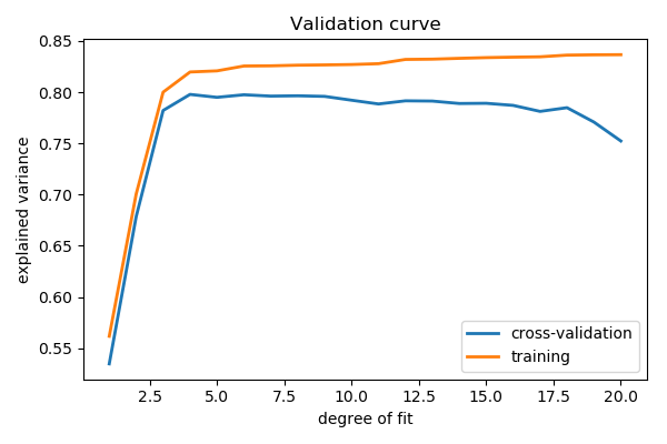
../../../_images/sphx_glr_plot_bias_variance_002.png

Plot a validation curve

 
   from sklearn.model_selection import validation_curve

degrees = np.arange(1, 21)

model = make_pipeline(PolynomialFeatures(), LinearRegression())

# The parameter to vary is the "degrees" on the pipeline step
# "polynomialfeatures"
train_scores, validation_scores = validation_curve(
                 model, x[:, np.newaxis], y,
                 param_name='polynomialfeatures__degree',
                 param_range=degrees)

# Plot the mean train error and validation error across folds
plt.figure(figsize=(6, 4))
plt.plot(degrees, validation_scores.mean(axis=1), lw=2,
         label='cross-validation')
plt.plot(degrees, train_scores.mean(axis=1), lw=2, label='training')

plt.legend(loc='best')
plt.xlabel('degree of fit')
plt.ylabel('explained variance')
plt.title('Validation curve')
plt.tight_layout()
 
  

../../../_images/sphx_glr_plot_bias_variance_003.png

Learning curves

Plot train and test error with an increasing number of samples

 
    # A learning curve for d=1, 5, 15
for d in [1, 5, 15]:
    model = make_pipeline(PolynomialFeatures(degree=d), LinearRegression())

    from sklearn.model_selection import learning_curve
    train_sizes, train_scores, validation_scores = learning_curve(
        model, x[:, np.newaxis], y,
        train_sizes=np.logspace(-1, 0, 20))

    # Plot the mean train error and validation error across folds
    plt.figure(figsize=(6, 4))
    plt.plot(train_sizes, validation_scores.mean(axis=1),
            lw=2, label='cross-validation')
    plt.plot(train_sizes, train_scores.mean(axis=1),
                lw=2, label='training')
    plt.ylim(ymin=-.1, ymax=1)

    plt.legend(loc='best')
    plt.xlabel('number of train samples')
    plt.ylabel('explained variance')
    plt.title('Learning curve (degree=%i)' % d)
    plt.tight_layout()


plt.show()
 
   

3.6.9.17. Tutorial Diagrams

This script plots the flow-charts used in the scikit-learn tutorials.

 
   import numpy as np
import pylab as pl
from matplotlib.patches import Circle, Rectangle, Polygon, Arrow, FancyArrow

def create_base(box_bg = '#CCCCCC',
                arrow1 = '#88CCFF',
                arrow2 = '#88FF88',
                supervised=True):
    fig = pl.figure(figsize=(9, 6), facecolor='w')
    ax = pl.axes((0, 0, 1, 1),
                 xticks=[], yticks=[], frameon=False)
    ax.set_xlim(0, 9)
    ax.set_ylim(0, 6)

    patches = [Rectangle((0.3, 3.6), 1.5, 1.8, zorder=1, fc=box_bg),
               Rectangle((0.5, 3.8), 1.5, 1.8, zorder=2, fc=box_bg),
               Rectangle((0.7, 4.0), 1.5, 1.8, zorder=3, fc=box_bg),

               Rectangle((2.9, 3.6), 0.2, 1.8, fc=box_bg),
               Rectangle((3.1, 3.8), 0.2, 1.8, fc=box_bg),
               Rectangle((3.3, 4.0), 0.2, 1.8, fc=box_bg),

               Rectangle((0.3, 0.2), 1.5, 1.8, fc=box_bg),

               Rectangle((2.9, 0.2), 0.2, 1.8, fc=box_bg),

               Circle((5.5, 3.5), 1.0, fc=box_bg),

               Polygon([[5.5, 1.7],
                        [6.1, 1.1],
                        [5.5, 0.5],
                        [4.9, 1.1]], fc=box_bg),

               FancyArrow(2.3, 4.6, 0.35, 0, fc=arrow1,
                          width=0.25, head_width=0.5, head_length=0.2),

               FancyArrow(3.75, 4.2, 0.5, -0.2, fc=arrow1,
                          width=0.25, head_width=0.5, head_length=0.2),

               FancyArrow(5.5, 2.4, 0, -0.4, fc=arrow1,
                          width=0.25, head_width=0.5, head_length=0.2),

               FancyArrow(2.0, 1.1, 0.5, 0, fc=arrow2,
                          width=0.25, head_width=0.5, head_length=0.2),

               FancyArrow(3.3, 1.1, 1.3, 0, fc=arrow2,
                          width=0.25, head_width=0.5, head_length=0.2),

               FancyArrow(6.2, 1.1, 0.8, 0, fc=arrow2,
                          width=0.25, head_width=0.5, head_length=0.2)]

    if supervised:
        patches += [Rectangle((0.3, 2.4), 1.5, 0.5, zorder=1, fc=box_bg),
                    Rectangle((0.5, 2.6), 1.5, 0.5, zorder=2, fc=box_bg),
                    Rectangle((0.7, 2.8), 1.5, 0.5, zorder=3, fc=box_bg),
                    FancyArrow(2.3, 2.9, 2.0, 0, fc=arrow1,
                               width=0.25, head_width=0.5, head_length=0.2),
                    Rectangle((7.3, 0.85), 1.5, 0.5, fc=box_bg)]
    else:
        patches += [Rectangle((7.3, 0.2), 1.5, 1.8, fc=box_bg)]

    for p in patches:
        ax.add_patch(p)

    pl.text(1.45, 4.9, "Training\nText,\nDocuments,\nImages,\netc.",
            ha='center', va='center', fontsize=14)

    pl.text(3.6, 4.9, "Feature\nVectors",
            ha='left', va='center', fontsize=14)

    pl.text(5.5, 3.5, "Machine\nLearning\nAlgorithm",
            ha='center', va='center', fontsize=14)

    pl.text(1.05, 1.1, "New Text,\nDocument,\nImage,\netc.",
            ha='center', va='center', fontsize=14)

    pl.text(3.3, 1.7, "Feature\nVector",
            ha='left', va='center', fontsize=14)

    pl.text(5.5, 1.1, "Predictive\nModel",
            ha='center', va='center', fontsize=12)

    if supervised:
        pl.text(1.45, 3.05, "Labels",
                ha='center', va='center', fontsize=14)

        pl.text(8.05, 1.1, "Expected\nLabel",
                ha='center', va='center', fontsize=14)
        pl.text(8.8, 5.8, "Supervised Learning Model",
                ha='right', va='top', fontsize=18)

    else:
        pl.text(8.05, 1.1,
                "Likelihood\nor Cluster ID\nor Better\nRepresentation",
                ha='center', va='center', fontsize=12)
        pl.text(8.8, 5.8, "Unsupervised Learning Model",
                ha='right', va='top', fontsize=18)



def plot_supervised_chart(annotate=False):
    create_base(supervised=True)
    if annotate:
        fontdict = dict(color='r', weight='bold', size=14)
        pl.text(1.9, 4.55, 'X = vec.fit_transform(input)',
                fontdict=fontdict,
                rotation=20, ha='left', va='bottom')
        pl.text(3.7, 3.2, 'clf.fit(X, y)',
                fontdict=fontdict,
                rotation=20, ha='left', va='bottom')
        pl.text(1.7, 1.5, 'X_new = vec.transform(input)',
                fontdict=fontdict,
                rotation=20, ha='left', va='bottom')
        pl.text(6.1, 1.5, 'y_new = clf.predict(X_new)',
                fontdict=fontdict,
                rotation=20, ha='left', va='bottom')

def plot_unsupervised_chart():
    create_base(supervised=False)


if __name__ == '__main__':
    plot_supervised_chart(False)
    plot_supervised_chart(True)
    plot_unsupervised_chart()
    pl.show() 
  

风吴痕

关注

0
点赞
踩
1

收藏

觉得还不错? 一键收藏
0
评论
Python3-sklearn

参考地址：1、http://www.scipy-lectures.org/packages/scikit-learn/index.html3.6. scikit-learn: machine learning in PythonSee also Data science in PythonThe Statistics in Pytho
复制链接

扫一扫

专栏目录