python3之sklearn示例学习

scikit-learn(含API) 是基于 Python 语言的机器学习工具
1.简单高效的数据挖掘和数据分析工具
2.可供大家在各种环境中重复使用
3.建立在 NumPy ，SciPy 和 matplotlib 上
4.开源，可商业使用 - BSD许可证

通用学习模式

from sklearn import datasets
from sklearn.model_selection import train_test_split
from sklearn.neighbors import KNeighborsClassifier

iris = datasets.load_iris()
iris_X = iris.data
iris_y = iris.target

X_train, X_test, y_train, y_test = train_test_split(
    iris_X, iris_y, test_size=0.3
)

knn = KNeighborsClassifier()
knn.fit(X_train, y_train)

print(knn.predict(X_test))  #训练后预测结果
print(y_test)               #真实的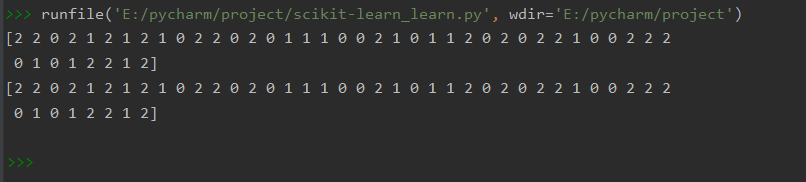结果

运行结果

from sklearn import datasets
from sklearn.linear_model import LinearRegression

loaded_data = datasets.load_boston()
data_X = loaded_data.data
data_y = loaded_data.target

model = LinearRegression()
model.fit(data_X, data_y)

print(model.predict(data_X[:4, :]))     #训练后预测结果
print(data_y[:4])                       #真实的结果

运行结果

sklearn 的 datasets 数据库

from sklearn import datasets
import matplotlib.pyplot as plt

# 生成回归模型的数据
X, y = datasets.make_regression(n_samples=100,
                                n_features=1,
                                #n_targets : int, optional (default=1) 参数
                                #The number of regression targets, i.e., 
                                #the dimension of the y output vector associated with a sample. 
                                #By default, the output is a scalar.
                                n_targets=1,
                                #noise : float, optional (default=0.0)参数
                                #The standard deviation of the gaussian noise applied to the output.
                                noise=10)
plt.scatter(X, y)
plt.show()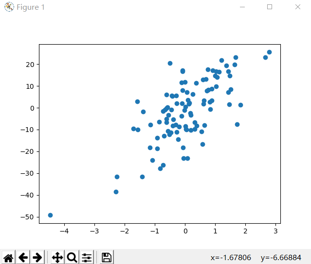

model 常用属性和功能

from sklearn import datasets
from sklearn.linear_model import LinearRegression

loaded_data = datasets.load_boston()
data_X = loaded_data.data
data_y = loaded_data.target

model = LinearRegression()
# LinearRegression().fit(self, X, y, sample_weight=None)
# X : array-like or sparse matrix, shape (n_samples, n_features)
# Training data
# y : array_like, shape (n_samples, n_targets)
# Target values. Will be cast to X’s dtype if necessary
model.fit(data_X, data_y)

print(model.coef_) 
# coef_ : array, shape (n_features, ) or (n_targets, n_features)
# Estimated coefficients for the linear regression problem. 
# If multiple targets are passed during the fit (y 2D), 
# this is a 2D array of shape (n_targets, n_features), 
# while if only one target is passed, this is a 1D array of length n_features.
print(model.intercept_)   #截距
# intercept_ : array
# Independent term in the linear model.

print(model.get_params())   #获得定义的参数

print(model.score(data_X, data_y)) 
# Returns the coefficient of determination R^2 of the prediction.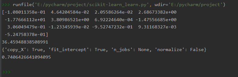

normalization 标准化数据

from sklearn import preprocessing
import numpy as np

a = np.array([[10, 2.7, 3.6],
             [-100, 5, -2],
             [120, 20, 40]], dtype=np.float64)

print(a)
print(preprocessing.scale(a))
# sklearn.preprocessing.scale(X, axis=0, with_mean=True, with_std=True, copy=True):
# axis used to compute the means(平均值) and standard deviations along. 
# If 0, independently standardize each feature, 
# otherwise (if 1) standardize each sample(样本).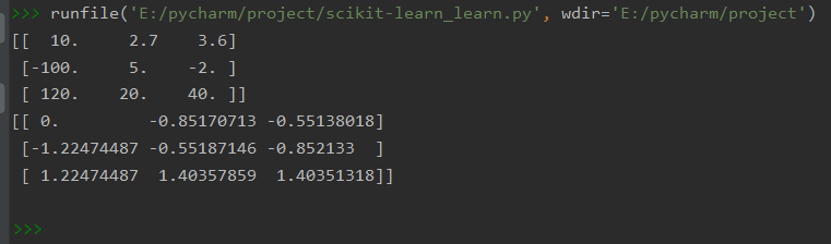

from sklearn import preprocessing
import numpy as np
from sklearn.model_selection import train_test_split
from sklearn.datasets.samples_generator import make_classification
from sklearn.svm import SVC
import matplotlib.pyplot as plt

# X : array of shape [n_samples, n_features]
#    The generated samples.
# y : array of shape [n_samples]
#    The integer labels for class membership of each sample.
X, y = make_classification(n_samples=300,
                           n_features=2,
                           n_redundant=0, 
                           #n_redundant:
                           # The number of redundant(冗余) features. These features are generated
                           #  as random linear combinations of the informative features.
                           n_informative=2, # n_informative : int, optional (default=2)
                           random_state=22,
                           n_clusters_per_class=1, 
                           # The number of clusters(簇) per class(类).(default=2)
                           scale=100)
# plt.scatter(X[:, 0], X[:, 1], c=y)
# plt.show()

X = preprocessing.minmax_scale(X, feature_range=(0, 1))
X_train, X_test, y_train, y_test = train_test_split(X, y, test_size=.3)
clf = SVC()
'''
sklearn.svm.SVC:
C-Support Vector Classification.

The implementation is based on libsvm. 
The fit time scales at least quadratically(平方比例) with the number of samples 
and may be impractical beyond tens of thousands of samples.
For large datasets consider using sklearn.linear_model.LinearSVC or 
sklearn.linear_model.SGDClassifier instead(代替), 
possibly after a sklearn.kernel_approximation.Nystroem transformer.

The multiclass support is handled(处理) according to a one-vs-one scheme(方案).
'''
clf.fit(X_train, y_train)
print(clf.score(X_test, y_test))
#0.9222222222222223 
#若没有用标准化则为0.4444444444444444

cross validation 交叉验证

from sklearn.datasets import load_iris
from sklearn.model_selection import train_test_split
from sklearn.neighbors import KNeighborsClassifier
from sklearn.model_selection import cross_val_score

iris = load_iris()
X = iris.data
y = iris.target

# #1.不加交叉验证
# X_train, X_test, y_train, y_test = train_test_split(X, y, random_state=4)
# knn = KNeighborsClassifier(n_neighbors=5)
# knn.fit(X_train, y_train)
# print(knn.score(X_test, y_test)) # 0.9736842105263158

#2.加交叉验证
knn = KNeighborsClassifier(n_neighbors=5)
scores = cross_val_score(knn, X, y, cv=5, scoring='accuracy')
print(scores) # [0.96666667 1.         0.93333333 0.96666667 1.        ]
print(scores.mean()) # 平均后 0.9733333333333334

from sklearn.datasets import load_iris
from sklearn.model_selection import train_test_split
from sklearn.neighbors import KNeighborsClassifier
from sklearn.model_selection import cross_val_score
import matplotlib.pyplot as plt

iris = load_iris()
X = iris.data
y = iris.target

k_range = range(1, 31)
k_scores = []

for k in k_range:
    knn = KNeighborsClassifier(n_neighbors=k)
    scores = cross_val_score(knn, X, y, cv=10, scoring='accuracy') # for classification
    k_scores.append(scores.mean())

plt.plot(k_range, k_scores)
plt.xlabel('Value of K for KNN')
plt.ylabel('Cross-Validated Accuracy')
plt.show()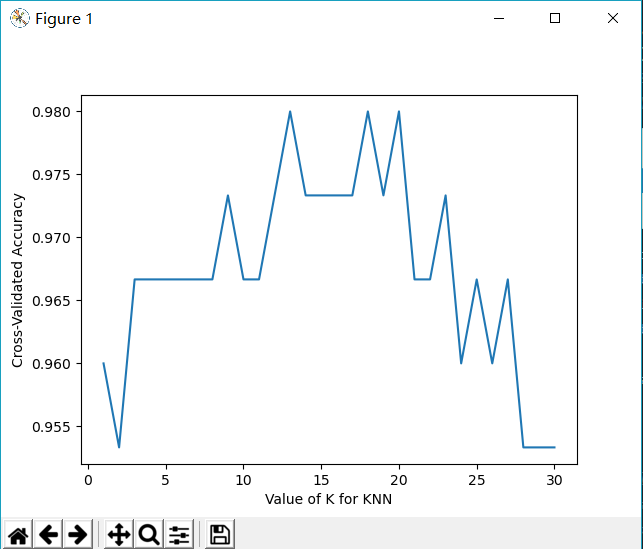

from sklearn.datasets import load_iris
from sklearn.model_selection import train_test_split
from sklearn.neighbors import KNeighborsClassifier
from sklearn.model_selection import cross_val_score
import matplotlib.pyplot as plt
import sklearn.metrics as metr

iris = load_iris()
X = iris.data
y = iris.target

k_range = range(1, 31)
k_scores = []

for k in k_range:
    knn = KNeighborsClassifier(n_neighbors=k)
    # print(metr.SCORERS.keys()) 查看scoring所有字段值
    loss = -cross_val_score(knn, X, y, cv=10, scoring='neg_mean_squared_error') # for regression
    k_scores.append(loss.mean())

plt.plot(k_range, k_scores)
plt.xlabel('Value of K for KNN')
plt.ylabel('Cross-Validated neg_mean_squared_error')
plt.show()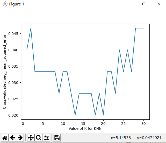

import matplotlib.pyplot as plt
from sklearn.model_selection import learning_curve
from sklearn.datasets import load_digits
from sklearn.svm import SVC
import numpy as np

digits = load_digits()
X = digits.data
y = digits.target

'''
Learning curve.
Determines cross-validated training and test scores for different training set sizes.
A cross-validation generator splits the whole dataset k times in training and test data. 
Subsets of the training set with varying sizes will be used to train the estimator 
and a score for each training subset size and the test set will be computed. 
Afterwards, the scores will be averaged over all k runs for each training subset size.
'''
train_sizes, train_loss, test_loss = learning_curve(
    SVC(gamma=0.001), X, y, cv=10,
    scoring='neg_mean_squared_error',
    train_sizes=[0.1, 0.25, 0.5, 0.75, 1]
)
'''
train_sizes : array-like, shape (n_ticks,), dtype float or int
Relative or absolute numbers of training examples that will be used to generate the learning curve. 
If the dtype is float, it is regarded as a fraction of the maximum size of 
the training set (that is determined by the selected validation method), i.e. 
it has to be within (0, 1]. Otherwise it is interpreted as absolute sizes of the training sets. 
Note that for classification the number of samples usually have to be big enough to contain 
at least one sample from each class. (default: np.linspace(0.1, 1.0, 5))
'''

train_loss_mean = -np.mean(train_loss, axis=1)
test_loss_mean = -np.mean(test_loss, axis=1)
'''
a = np.array([[1, 2], [3, 4]])
print(np.mean(a))     # 对所有元素求均值 -> 2.5
print(np.mean(a, 0))  # 压缩行，对各列求均值  -> [2. 3.]
print(np.mean(a, 1))  # 压缩列，对各行求均值  -> [1.5 3.5]
'''

plt.plot(train_sizes, train_loss_mean,
         'o-', color='r', label='Training')
plt.plot(train_sizes, test_loss_mean,
         'o-', color='g', label='Cross-validation')

plt.xlabel('Training examples')
plt.ylabel('Loss')
plt.legend(loc='best')
plt.show()

import matplotlib.pyplot as plt
from sklearn.model_selection import validation_curve
from sklearn.datasets import load_digits
from sklearn.svm import SVC
import numpy as np

digits = load_digits()
X = digits.data
y = digits.target

param_range = np.logspace(-6, -2.3, 5)
'''
numpy.logspace(开始点，结束点，总数)
开始点和结束点是10的幂
'''
train_loss, test_loss = validation_curve(
    SVC(), X, y,
    param_name='gamma', param_range=param_range,
    cv=10, scoring='neg_mean_squared_error',
)
'''
Validation curve.
Determine training and test scores for varying parameter values.
Compute scores for an estimator with different values of a specified parameter. 
This is similar to grid search with one parameter. 
However, this will also compute training scores and is merely a utility for plotting the results.
'''

train_loss_mean = -np.mean(train_loss, axis=1)
test_loss_mean = -np.mean(test_loss, axis=1)

plt.plot(param_range, train_loss_mean,
         'o-', color='r', label='Training')
plt.plot(param_range, test_loss_mean,
         'o-', color='g', label='Cross-validation')

plt.xlabel('gamma')
plt.ylabel('Loss')
plt.legend(loc='best')
plt.show()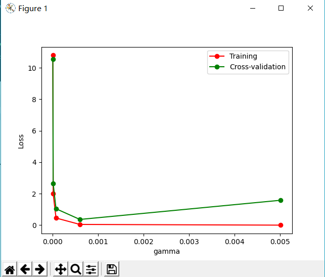

Save

from sklearn import svm
from sklearn import datasets

clf = svm.SVC()
iris = datasets.load_iris()
X, y = iris.data, iris.target
clf.fit(X, y)

# method 1: pickle
import pickle
with open('save/clf.pickle', 'wb') as f:
    pickle.dump(clf, f)

# # 注释以上保存文件的代码和训练代码运行
# with open('save/clf.pickle', 'rb') as f:
#     clf2 = pickle.load(f)
#     print(clf2.predict(X[0:1]))

from sklearn import svm
from sklearn import datasets

clf = svm.SVC()
iris = datasets.load_iris()
X, y = iris.data, iris.target
clf.fit(X, y)

# method 2: joblib
from sklearn.externals import joblib

joblib.dump(clf, 'save/clf.pkl') # save

clf3 = joblib.load('save/clf.pkl') # restore
print(clf3.predict(X[0:1]))

参考：Scikit-learn (sklearn) 优雅地学会机器学习 (莫烦 Python 教程)