dbscan js 实现_DBSCAN在PySpark上的实现

最新推荐文章于 2024-08-15 10:01:45 发布

weixin_26632369

最新推荐文章于 2024-08-15 10:01:45 发布

阅读量632

点赞数 1

文章标签： java python

原文链接：https://towardsdatascience.com/an-efficient-implementation-of-dbscan-on-pyspark-3e2be646f57d

版权

本文介绍了如何高效地在PySpark上实现DBSCAN聚类算法，并提到了JavaScript版本的DBSCAN实现。

摘要由CSDN通过智能技术生成

dbscan js 实现

DBSCAN is a well-known clustering algorithm that has stood the test of time. Though the algorithm is not included in Spark MLLib. There are a few implementations (1, 2, 3) though they are in scala. Implementation in PySpark uses the cartesian product of rdd to itself which results in O(n²) complexity and possibly O(n²) memory before the filter.

DBSCAN是一种久经考验的著名聚类算法。尽管该算法未包含在Spark MLLib中。有几个实现( 1 ， 2 ， 3 )，尽管它们在阶。在PySpark中的实现将rdd的笛卡尔积用于自身，这会导致O(n²)复杂性，并可能在过滤器之前存储O(n²)内存。

ptsFullNeighborRDD=rdd.cartesian(rdd)                            .filter(lambda (pt1,pt2): dist(pt1,pt2)<eps)                            .map(lambda (pt1,pt2):(pt1,[pt2]))                            .reduceByKey(lambda pts1,pts2: pts1+pts2)                            .filter(lambda (pt, pts): len(pts)>=minPts)source: https://github.com/htleeab/DBSCAN-pyspark/blob/master/DBSCAN.py

For a quick primer on the complexity of the DBSCAN algorithm:

要快速了解DBSCAN算法的复杂性，请执行以下操作：

https://en.wikipedia.org/wiki/DBSCAN#Complexity

https://zh.wikipedia.org/wiki/DBSCAN#复杂度

DBSCAN visits each point of the database, possibly multiple times (e.g., as candidates to different clusters). For practical considerations, however, the time complexity is mostly governed by the number of regionQuery invocations. DBSCAN executes exactly one such query for each point, and if an indexing structure is used that executes a neighborhood query in O(log n), an overall average runtime complexity of O(n log n) is obtained (if parameter ε is chosen in a meaningful way, i.e. such that on average only O(log n) points are returned). Without the use of an accelerating index structure, or on degenerated data (e.g. all points within a distance less than ε), the worst case run time complexity remains O(n²). The distance matrix of size (n²-n)/2 can be materialized to avoid distance recomputations, but this needs O(n²) memory, whereas a non-matrix based implementation of DBSCAN only needs O(n) memory.

DBSCAN可能会多次访问数据库的每个点(例如，作为不同群集的候选项)。但是，出于实际考虑，时间复杂度主要取决于regionQuery调用的次数。 DBSCAN对每个点仅执行一个这样的查询，如果使用索引结构在O(log n )中执行邻域查询，则将获得O( n log n )的总体平均运行时复杂度(如果在一种有意义的方式，即平均仅返回O(log n )点)。无需使用加速索引结构的，或对退化的数据(例如距离小于ε内的所有点)，最坏的情况下运行时间复杂度保持为O(n²)。 大小(N²-n)的距离基质/ 2可以被物化，以避免距离recomputations，但这需要为O(n²)存储器，而DBSCAN的非基于矩阵的实现仅需要O(n)的存储器中。

In this post, we will explore how we can implement DBSCAN in PySpark efficiently without using O(n²) operations by reducing the number of distance calculations. We would implement an indexing/partitioning structure based on Triangle Inequality to achieve this.

在这篇文章中，我们将探讨如何通过减少距离计算的次数而在不使用O(n²)操作的情况下有效地在PySpark中实现DBSCAN。我们将基于三角不等式实现索引/分区结构以实现此目的。

三角不等式 (Triangle Inequality)

Let’s refresh triangle inequality. If there are three vertices of the triangle a, b and c, and given distance metric d. Then

让我们刷新三角形不等式。如果存在三角形a ， b和c的三个顶点，并且给定距离度量d。然后

d(a, b) ≤ d(a, c) + d(c, b)

d ( a，b ) ≤d(A，C)+ d(C，B)

d(a, c) ≤ d(a, b) + d(b, c)

d ( a，c ) ≤d(A，B)+ d(B，C)

d(b, c) ≤ d(b, a) + d(a, c)

d ( b，c ) ≤d(B，A)+ d(A，C)

In DBSCAN there is a parameter ε, which is used to find the linkage between points. Now, let us use this parameter to see if we can use triangle inequality to reduce the number of operations.

在DBSCAN中，存在一个参数ε，该参数用于查找点之间的链接。现在，让我们使用此参数来查看是否可以使用三角不等式来减少运算次数。

Let’s say there are four points x, y, z, and c.

假设x ， y，z和c有四个点。

Lemma 1: If d(x, c) ≥ (k+1)ε and d(y, c) < kε then d(x, y) > ε

引理1：如果d(X，C)≥(K +1)ε和d(Y，C)<Kε则d(X，Y)>ε

As per triangle inequality,

根据三角形不等式，

d(x, c) ≤ d(x, y) + d(y, c)

d(X，C)≤d(X，Y)+ d(Y，C)

d(x, c)-d(y, c)≤ d(x, y)

d(X，C) - d(Y，C)≤d(X，Y)

d(x, c)-d(y, c) > (k+1)ε -kε > ε

d(X，C) - d(Y，C)>(K +1)ε - Kε>ε

so d(x, y) > ε

所以d ( x，y )>ε

Lemma 2: If d(x, c) ≤ lε and d(z, c) > (l+1)ε then d(x, z) > ε

引理2：如果d(X，C)≤ 升 ε和d(Z，C)>(L + 1)ε则D(X，Z)>ε

As per triangle inequality,

根据三角形不等式，

d(z, c) ≤ d(x, z) + d(x, c)

d(Z，C)≤d(X，Z)+ d(X，C)

d(z, c)-d(x, c)≤ d(x, z)

d(Z，C) - d(X，C)≤d(X，Z)

d(z, c)-d(x, c) > (l+1)ε -lε

d(Z，C) - d(X，C)>(L 1)ε - 升 ε

d(z, c)-d(x, c) > ε

d ( z，c ) -d ( x，c )>ε

so d(x, z) > ε

所以d ( x，z )>ε

What we can deduce from above is that if we compute distances of all points from c then we can filter points y and z using above criteria. We can compute distances from c and partition points in concentric rings (center being c).

我们可以从上面得出的结论是，如果我们计算所有点与c的距离，则可以使用上述准则对点y和z进行过滤。我们可以计算出与c和同心环(中心为c )中的分隔点的距离。

重叠的同心环分区 (Overlapping Concentric Ring Partitions)

分区的宽度应该是多少？ (What should be the width of the partitions?)

From the above lemmas, we can see that if

从上面的引理，我们可以看到

(m+1)ε ≥ d(x, c) ≥ mε then we can filter out points y and z if d(y, c) < (m-1)ε and d(z, c) > (m+2)ε

第(m + 1)ε≥d(X，C)≥ 米 ε那么我们可以过滤掉点y和z如果d(Y，C)<( 米 -1)ε和d(Z，C)>(M + 2) ε

From this, we can deduce that for any point for which (m+1)ε ≥ d(x, c) ≥ mε is true we can have a partition of (m+3)ε width starting at (m-1)ε and ending at (m+2)ε.

由此，我们可以推断出，对于任何点，其第(m + 1)ε≥d(X，C)≥ 米 ε为真，我们可以具有(M 3)的分隔ε宽度从(m -1) 个 ε并以( m + 2)ε结束。

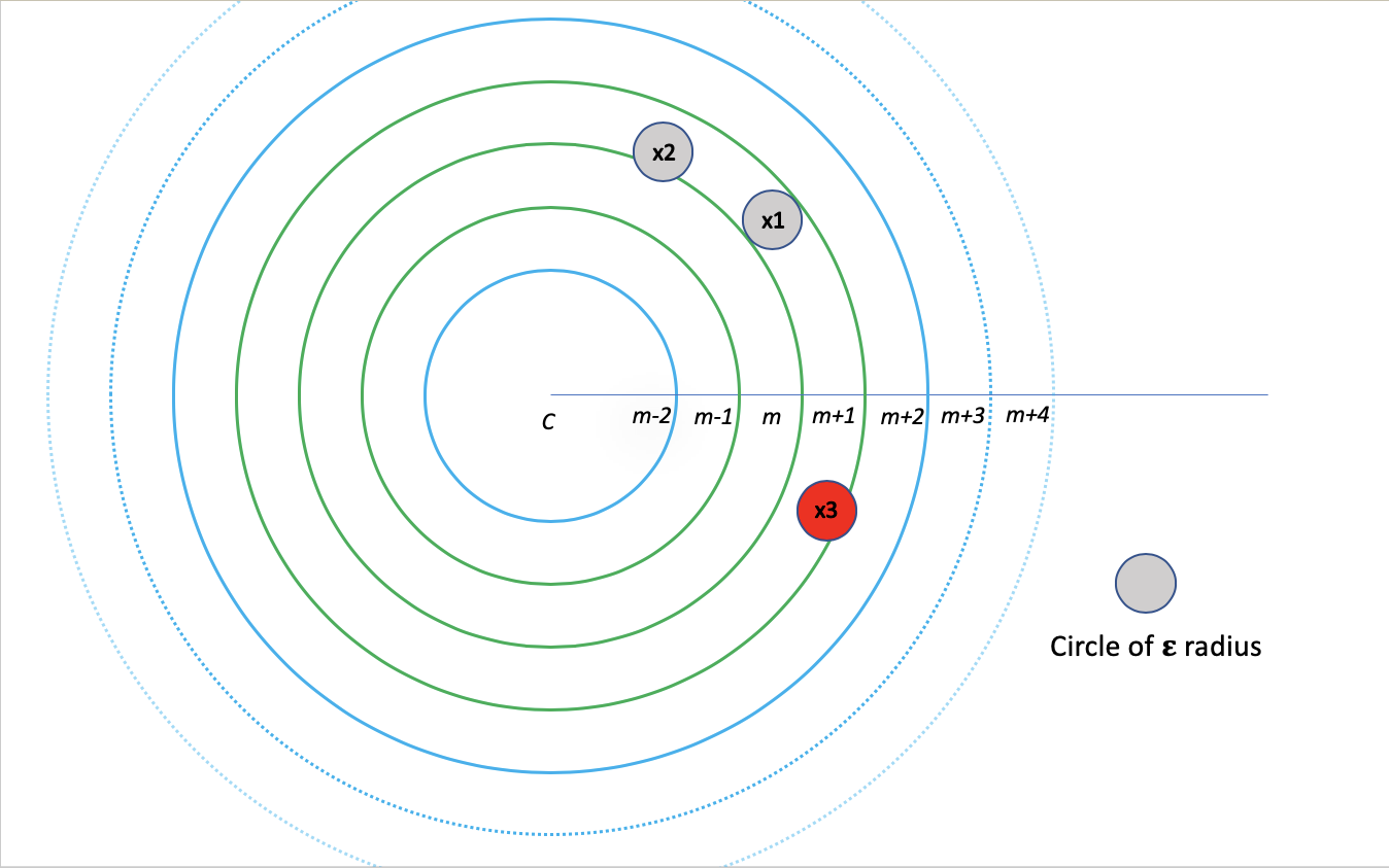
Here is a depiction how it would look like. Two-dimensional space is divided into quantiles of ε euclidean distance. Green rings show the partition. x1 is at the (m+1/2)ε distance from c (center of (m-1)ε — (m+2)ε partition). x2 and x3 are at mε and (m+1)ε distance from c. It is clear that for x1, x2, and x3 all points of relevance (within the circle of radius ε) are within the partition.

这是它的外观描述。二维空间分为ε欧式距离的分位数。绿色环显示该分区。 x 1距c (( m- 1 ) ε-( m +2)ε分区的中心)为( m +1/2)ε距离。 X 2和X 3是在m和ε(M 1)从Cε距离。显然，对于x 1， x 2和x 3，所有相关点(在半径ε的圆内)都在分区内。

If we create mutually exclusive partitions and compute distances among points within that partition, it would be incomplete. For example, x4 and x5’s range circle will overlap two partitions. Hence the need for overlapping partition. One strategy could be to move the partition by ε. Though in that case if partition width is 3ε, then one point may occur in three different partitions. Instead, partitions are created of 2ε width and move them by ε. In this case, one point may occur only in two partitions.

如果我们创建互斥分区，并计算该分区内各点之间的距离，则将是不完整的。例如， x 4和x 5的范围圆将与两个分区重叠。因此需要重叠分区。一种策略可能是将分区移动ε。尽管在这种情况下，如果分隔宽度为3ε，则在三个不同的分隔中可能会出现一个点。而是创建宽度为2ε的分区，并将其移动ε。在这种情况下，一个点可能仅出现在两个分区中。

The above two images show how this partition scheme works. Two partitions in combination allow a range query of ε radius for all the points from mε to (m+1)ε. The first partition covers all the points from mε to (m+1/2)ε (x2 covered but x3 not) and the second covers (m+1/2)ε to (m+1)ε (x3 covered but x2 not).

上面的两个图像显示了此分区方案的工作方式。在组合的两个分区允许ε半径的所有从米 ε至(m + 1)ε的点的范围的查询。第一分区覆盖的所有点从米 ε至(m + 1/2)ε(×2覆盖，但×3不)和第二盖(M + 1/2)ε至(m + 1)ε(×3覆盖，而X 2不是)。

分区可视化 (Partitioning Visualization)

Let us see how these partitions look like on some generated data.

让我们看看这些分区在某些生成的数据上的样子。

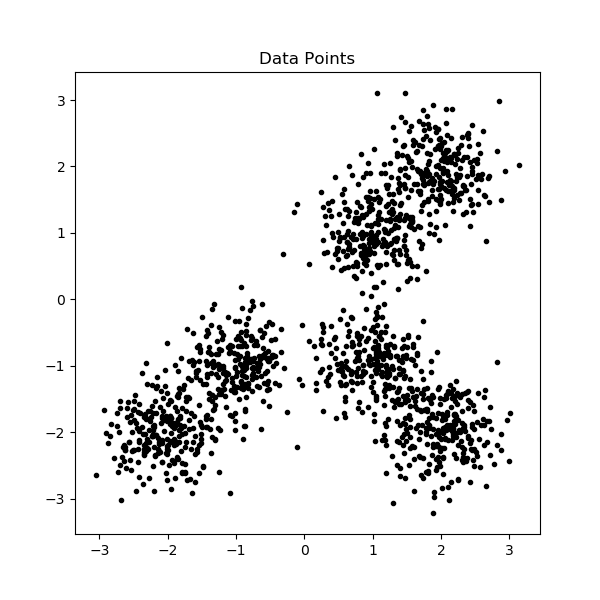
The above data and image are generated by the following code:

以上数据和图像由以下代码生成：

The above partitions from data are generated by the following code:

上面的数据分区是由以下代码生成的：

partition_index identifies each partition. Each data point is put into two partitions as discussed before based on the distance from c (pivot) and ε. distance method handles one point at a time. In PySpark flatMap method is used to map every point into an array of tuples (out).

partition_index标识每个分区。如前所述，根据与c (枢轴)和ε的距离，将每个数据点分为两个分区。距离法一次只能处理一个点。在PySpark中， flatMap方法用于将每个点映射到元组数组(输出)。

合并分区 (Merging Partitions)

All data points within a partition are merged before generating the visualization. They also need to be merged for further processing DBSCAN on PySpark.

在生成可视化文件之前，将合并分区中的所有数据点。它们也需要合并，以便在PySpark上进一步处理DBSCAN。

reduceByKey method is used to merge partition data in one. The use of word partition may confuse with PySpark partitions but those are two separate things. Though partitionBy method could be used to reconcile that as well.

reduceByKey方法用于合并分区数据。单词分区的使用可能会与PySpark分区混淆，但这是两个不同的东西。尽管partitionBy方法也可以用来协调它。

After reduceByKey, we will get each row of the rdd as a ring depicted in figure 4. As you can see there is an overlap so points would be in two rows of rdd and that is intentional.

在reduceByKey之后，我们将得到rdd的每一行，如图4所示。如您所见，有一个重叠部分，所以点将位于rdd的两行中，这是有意的。

距离计算 (Distance Calculations)

The above code computes distance within each partition. The output of the method is a list of tuples. Each tuple has the id of point and set of its neighbors within ε distance. As we know that point would occur in two partitions so we need to combine the sets for a given point so we get all of its neighbors within ε distance in whole data. reduceByKey is used to combine the sets by doing union operation on them.

上面的代码计算每个分区内的距离。该方法的输出是一个元组列表。每个元组在ε距离内具有点的ID和其邻居的集合。我们知道该点将出现在两个分区中，因此我们需要组合给定点的集合，以便在整个数据中获得ε距离内的所有邻居。 reduceByKey用于通过对集合进行联合操作来组合集合。

reduceByKey(lambda x, y: x.union(y))

Combined code till now looks as follows:

到目前为止，组合的代码如下所示：

核心和边界点标签 (Core and Border Point Labeling)

Once we have neighbors within ε distance for a point we can identify if it is a core or border point.

一旦我们在一个点的ε距离内有邻居，就可以确定它是核心点还是边界点。

Core Point: There are at least min_pts within ε distance

核心点 ：ε距离内至少有min_pts

Border Point: There are less than min_pts within ε distance but one of them is the core point.

边界点 ：ε距离内的min_pts小于，但其中之一是核心点。

To identify core and border points, first, we assign them to a cluster. For each point which is a core point, we create a cluster label the same to its id (assuming the ids are unique). We create a tuple for each core point and its neighbors of the form (id, [(cluster_label, is_core_point)]). All the neighbors in this scenario would be labeled as a base point. Let's take an example

为了识别核心和边界点，首先，我们将它们分配给一个群集。对于作为核心点的每个点，我们都创建一个与其ID相同的群集标签(假设ID是唯一的)。我们为每个核心点及其邻居创建一个元组，形式为( id ，[( cluster_label ， is_core_point )])。在这种情况下，所有邻居都将被标记为基点。让我们举个例子

min_pts = 3
Input: (3, set(4,6,2))
Output: [(3, [(3, True)]), (4, [(3, False)]), (6, [(3, False)]), (2, [(3, False)])]

Input is a tuple where 3 is the id of point and (4, 6, 2) are its neighbors within ε distance.

输入是一个元组，其中3是点的id，(4，6，2)是其在ε距离内的邻居。

As one can see all points are assigned cluster label 3. While 3 is assigned True for is_core_point as a core point and all other points are considered base points and assigned False for is_core_point.

如可以看到的所有点被分配簇标签3.在3被分配为真 is_core_point作为核心点和所有其它点被认为基点和分配False的is_core_point。

We may have similar input tuples for 4, 6, and 2 where they may or may not be assigned as core points. The idea is to eventually combine all cluster labels for a point and if at least one of the assignment for is_core_point is True then its a core point otherwise its a border point.

对于4、6和2，我们可能有相似的输入元组，其中它们可能被分配或可能未被分配为核心点。想法是最终将所有聚类标签合并为一个点，如果is_core_point的分配中至少有一个为True，则其为核心点，否则为边界点。

We combine all (cluster_label, is_core_point) tuples for a point using reduceByKey method and then investigate if its a core point or not while combining all clusters labels for that point. If its a border point then we would only leave one cluster label for it.

我们使用reduceByKey方法将所有( cluster_label ， is_core_point )元组合并为一个点，然后在合并该点的所有聚类标签时研究其是否是核心点。如果它是一个边界点，那么我们将只为其保留一个群集标签。

The above method is used to combine all cluster label for a point. Again if it is a border point then we return only 1st cluster label.

上面的方法用于合并一个点的所有聚类标签。同样，如果它是一个边界点，那么我们仅返回第一个簇标签。

Code in PySpark till now looks like the following:

到目前为止，PySpark中的代码如下所示：

连接的核心和边界点 (Connected Core and Border Points)

Now for each point, we have cluster labels. If a point has more than one cluster label then it means those clusters are connected. Those connected clusters are the final clusters we need to solve DBSCAN. We solve this by creating a graph with vertices as cluster labels and edges between cluster labels if they are assigned to the same point.

现在，对于每个点，我们都有聚类标签。如果一个点具有多个群集标签，则表示这些群集已连接。这些连接的集群是解决DBSCAN所需的最终集群。为了解决这个问题，我们创建了一个图，该图的顶点作为聚类标签，而聚类标签之间的边(如果它们被分配给同一点)。

In the above code, combine_cluster_rdd is a collection of rows where each row is a tuple (point, cluster_labels). Each cluster label is vertices and combinations of cluster labels for a point are the edges. Connected components of this graph give a mapping between each cluster label and a connected cluster. which we can apply to points to get final clusters.

在上面的代码中，Combine_cluster_rdd是行的集合，其中每一行都是一个元组( point ， cluster_labels )。每个聚类标签是顶点，并且一个点的聚类标签的组合是边。该图的连接组件在每个群集标签和连接的群集之间提供了映射。我们可以将其应用于点以获得最终聚类。

Above is how the final method looks like which returns a Spark Dataframe with point id, cluster component label, and a boolean indicator if its a core point.

上面是最终方法的外观，该方法返回带有点ID，集群组件标签和布尔指示符(如果它是核心点)的Spark Dataframe。

比较 (Comparision)

Now I compare the results in terms of accuracy with sklearn implementation of DBSCAN.

现在，我将比较准确性与使用DBSCAN的sklearn实现的结果。

The make_blobs method creates blobs around three input centers. Running DBSCAN using sklearn and my implementation with ε=0.3 and min_pts=10 gives the following results.

make_blobs方法在三个输入中心周围创建斑点。使用sklearn和我的实现(其中ε= 0.3和min_pts = 10)运行DBSCAN可获得以下结果。

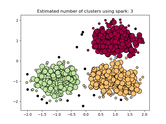
Core points are bigger circles while border points are smaller ones. Noise points are colored black which is the same in both implementations. One thing that jumps out is the border points are assigned different clusters that speak to the non-deterministic nature of DBSCAN. My other post also talks about it.

核心点是较大的圆圈，而边界点是较小的圆圈。噪声点被涂成黑色，这在两种实现中都是相同的。跳出的一件事是为边界点分配了不同的簇，这些簇说明了DBSCAN的不确定性。我的其他帖子也谈到了这一点。

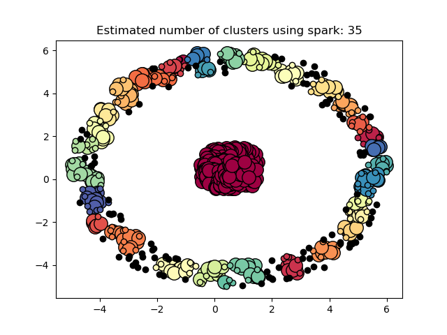
For ε=0.2 we get the border points assigned to the same clusters. Following is some code and results on data in rings.

对于ε= 0.2，我们获得分配给相同聚类的边界点。以下是一些代码和有关环数据的结果。

操作次数 (Number of Operations)

For n=750, the number of distance operations required by a simple implementation of DBSCAN would be n(n-1)/2 which is 280875. As we create the partition based on ε, the smaller the ε less the number of distance operations would be needed. In this case, there were a total of 149716(ε=.2) and 217624(ε=0.3) operations needed.

对于n = 750，简单实现DBSCAN所需的距离运算次数将为n(n-1)/ 2，即280875。当我们基于ε创建分区时，ε越小，距离运算次数越少将需要。在这种情况下，总共需要进行149716(ε= .2)和217624(ε= 0.3)运算。

振铃数据比较 (Comparison of Ring Data)

结论 (Conclusion)

A pyspark implementation which would be efficient based on the value of ε with the following steps:

一个基于ε值的pyspark实现，将执行以下步骤：

Partitioning Data: Partition with overlapping rings of 2ε width moved by ε.
分区数据：具有2ε宽度的重叠环移动ε的分区。
Merging Partition Data: So we get all partition data in a single record.
合并分区数据：因此，我们在单个记录中获取所有分区数据。
Distance Calculations: Calculate distance within the same partition
距离计算：计算同一分区内的距离
Point Labeling: Based on the number of neighbors, label core, and border points.
点标签：基于邻居的数量，标签核心和边界点。
Connected Clusters: Use Graphframe to connect clusters labels to evaluate final DBSCAN labels.
连接的群集：使用Graphframe连接群集标签以评估最终的DBSCAN标签。

A comparison with the existing implementation shows the accuracy of the algorithm and the implementation of this post.

与现有实现的比较显示了该算法的正确性以及本文的实现。

有效率吗？ (Is it efficient?)

On the local machine with both driver and worker nodes, implementation is slower than sklearn. There could be a couple of reasons which need to be investigated:

在具有驱动程序节点和工作程序节点的本地计算机上，实现比sklearn慢。可能有两个原因需要调查：

For a small amount of data, sklearn may be much faster but is it the case for big-data?
对于少量数据，sklearn可能会快得多，但是大数据是否是如此？
Graphframe takes quite some time to execute and wondering if connected components analysis can be performed on the driver with some other graph library?
Graphframe需要花费很多时间来执行，并且想知道是否可以使用其他图形库在驱动程序上执行连接组件分析？