x射线计算机断层成像_医疗保健中的深度学习-X射线成像（第4部分-类不平衡问题）...

x射线计算机断层成像

As we saw in the previous part — Part 3 — (https://towardsdatascience.com/deep-learning-in-healthcare-x-ray-imaging-part-3-analyzing-images-using-python-915a98fbf14c), the chest x-ray dataset has an imbalance of images. This is the bar chart of the images per class that we had seen in the previous part.

正如我们在上一部分(第3部分)中所看到的( https://towardsdatascience.com/deep-learning-in-healthcare-x-ray-imaging-part-3-analyzing-images-using-python-915a98fbf14c )，胸部X射线数据集的图像不平衡。 这是我们在上一部分中看到的每类图像的条形图。

In medical imaging datasets, this is a very common problem. Since most often the data is collected from various different sources, and not all diseases are as prevalent as others, so the datasets are imbalanced more often than not.

在医学成像数据集中，这是一个非常普遍的问题。 由于大多数情况下都是从各种不同的来源收集数据，而且并非所有疾病都像其他疾病一样普遍，因此数据集经常失衡。

So what is the problem if we train the neural network on an imbalanced dataset? The answer is that the network tends to learn more from the classes with more images than the ones with fewer images. That is, in this case, the model might predict more images to be ‘Bacterial Pneumonia’, even though the images might be from the other two classes, and that is an undesirable outcome when dealing with medical images.

那么，如果我们在不平衡的数据集上训练神经网络，会出现什么问题呢？ 答案是，网络倾向于从图像较多的类别中学习更多，而不是图像较少的类别。 也就是说，在这种情况下，即使图像可能来自其他两个类别，模型也可能会预测更多图像为“细菌性肺炎”，这在处理医学图像时是不希望的结果。

Also, it should be noted, while dealing with medical images, the final accuracy (both train accuracy or validation accuracy) of the model is not the right parameter to base the model’s performance on. Because, even if the model is performing poorly on a particular class, but performing well on the class with maximum images, the accuracy would still be high. In reality, we want the model to perform well in all the classes. Thus, there are other parameters, such as sensitivity(Recall/True Positive Rate (TPR)), specificity(True Negative Rate(TNR), Precision or Positive Predicted Value (PPV), and F-scores, which should be considered to analyze the performance of a trained model. We will discuss these in detail in a later part, where we discuss the confusion matrix.

另外，应注意，在处理医学图像时，模型的最终精度(训练精度或验证精度)不是基于模型性能的正确参数。 因为即使模型在特定类别上的表现不佳，但在具有最大图像的类别上表现良好，其准确性仍然很高。 实际上，我们希望模型在所有类中都能表现良好。 因此，应考虑其他参数，例如灵敏度(召回率/真实阳性率(TPR))，特异性(真实阴性率(TNR)，精确度或阳性预测值(PPV)和F得分)。训练模型的性能，我们将在后面的部分中详细讨论这些问题，并讨论混淆矩阵。

It is also a must to maintain a separate set of images, on which the model is neither trained nor validated, so as to check how the model performs on images that it has never seen before. This is also a compulsory step to analyze the performance of the model.

还必须维护一个单独的图像集，在该图像集上既未对其进行训练也未对其进行验证，以便检查该模型如何处理从未见过的图像。 这也是分析模型性能的必要步骤。

解决班级失衡的各种方法： (Various ways to tackle class imbalance:)

There are various ways to tackle the class imbalance problem. The best method is to collect more images for the minority classes. But that is not possible in certain situations. In that case, commonly these 3 methods can be beneficial: a. Weighted Loss b. Undersampling c. Oversampling

有多种方法可以解决班级不平衡问题。 最好的方法是为少数群体收集更多图像。 但这在某些情况下是不可能的。 在那种情况下，通常这三种方法可能是有益的： 加权损失 b。 欠采样 c。 过采样

We will go through each of these methods in details:

我们将详细介绍以下每种方法：

1. Updating the loss function — Weighted Loss

   更新损失函数-加权损失

Suppose we are using Binary Cross-Entropy loss function. The loss function looks like this -

假设我们正在使用二进制交叉熵损失函数 。 损失函数看起来像这样-

L(X,y) = - log P(Y =1 |X) if y =1 and -log P(Y=0 |X) if y=0

L(X，y)=-如果y = 1，则记录P(Y = 1 | X)；如果y = 0，则-log P(Y = 0 | X)

This measures the output of a classification model whose output is between zero and one. (This loss function only works if we are doing a binary classification problem. For multiple classes, we use Categorical Cross-Entropy loss or Sparse Categorical Cross-Entropy loss. We will discuss basic loss functions in a later part).

这将测量分类模型的输出，该模型的输出介于零和一之间。 (仅当我们正在执行二进制分类问题时，此损失函数才有效。对于多个类，我们使用分类交叉熵损失或稀疏分类交叉熵损失。我们将在后面的部分中讨论基本损失函数)。

Example — If the label of an image is 1, and the neural network algorithm predicts the probability that the label is 1 is 0.2.

示例—如果图像的标签为1，并且神经网络算法预测标签为1的概率为0.2。

Let's apply the loss function to compute the loss for this example. Notice that we are interested in the label 1. So, we are going to use the first part of the loss function L. The loss L is going to be -

在本示例中，我们应用损失函数来计算损失。 请注意，我们对标签1感兴趣。因此，我们将使用损失函数L的第一部分。损失L将为-

L =-log 0.2 = 0.70

L =对数0.2 = 0.70

So this is the loss the algorithm gets for this example.

因此，这就是算法在此示例中获得的损失。

For another image whose label is 0, if the algorithm predicts that the probability of the image to be label 0 is 0.7, then we use the second part of the loss function, but we cannot really use it directly. Rather we use a different approach. We know the maximum probability can be 1, so we calculate the probability of the label is 1.

对于另一个标签为0的图像，如果算法预测该图像被标记为0的概率为0.7，则我们使用损失函数的第二部分，但实际上不能直接使用它。 相反，我们使用不同的方法。 我们知道最大概率可以为1，因此我们计算标签的概率为1。

In this case, L = -log (1–0.7) =-log (0.3) = 0.52

在这种情况下，L = -log(1-0.7)= -log(0.3)= 0.52

Now let's look at multiple examples, with class imbalance.

现在让我们看一下带有类不平衡的多个示例。

Figure 1. Class Imbalance, Probability and Calculated loss (Source: Image created by author)

图1.类不平衡，概率和计算的损失(来源：作者创建的图像)

In Figure 1, we see there are a total of 10 images, but 8 of those belong to class label 1, and only two belong to class label 0. Hence this is a classic class imbalance problem. Assuming all were predicted with a probability 0.5,

在图1中，我们看到总共有10张图像，但是其中8张图像属于类标签1，只有两张图像属于类标签0。因此，这是经典的类不平衡问题。 假设所有预测的概率为0.5，

Loss L for label 1 = -log(0.5) = 0.3,

标签1的损耗L = -log(0.5)= 0.3，

Loss L for label 0 = -log(1–0.5) = -log(0.5) = 0.3

标签0的损耗L = -log(1-0.5)= -log(0.5)= 0.3

So, the total loss for label 1 = 0.3 x 8 = 2.4

因此，标签1的总损失= 0.3 x 8 = 2.4

whereas, the total loss for label 0 = 0.3 x 2 = 0.6

而标签0的总损失= 0.3 x 2 = 0.6

So, most of the contributions to the loss is coming from class with label 1. So the algorithm when updating weights will prefer to update weights of label 1 images much more, than weights of images with label 0. This does not produce a very good classifier, and this is the Class Imbalance Problem.

因此，对损失的大部分贡献来自标签1的类。因此，更新权重时的算法比标签0的图像权重更愿意更新标签1图像的权重。分类器，这是类不平衡问题 。

The solution to the class imbalance problem is to modify the loss function, to weigh the 1 and 0 classes differently.

解决类不平衡问题的方法是修改损失函数，对1类和0类进行加权 。

w1 is the weights we assign to label 1 examples, and w0 to label 0 examples. New Loss Function,

w1是我们分配给标签1示例的权重，w0是我们分配给标签0示例的权重。 新的损失函数

L = w1 x -log(Y =1 |X) if y =1 ,and,

如果y = 1，则L = w1 x -log(Y = 1 | X)

L = w0 x -log P(Y=0 |X) if y=0

如果y = 0，则L = w0 x -log P(Y = 0 | X)

We want to give more weights to classes with fewer images than the classes with more images. So in this case we give class 1 which as 8 examples a weight of 2/10 = 0.2, and class 0 which as 2 examples a weight of 8/10 = 0.8.

我们希望给图像较少的类更多的权重。 因此，在这种情况下，我们给出1类(作为8个示例，权重为2/10 = 0.2)和0类(作为2个示例，权重为8/10 = 0.8)。

Generally, the weights are calculated using the formula below,

通常，权重是使用以下公式计算的，

w1 = number of images with label 0/total number images = 2/10

w1 =带有标签0的图像数/总图像数= 2/10

w0 = number of images with label 1/total number of images = 8/10

w0 =带有标签1的图像数/图像总数= 8/10

Below is the updated table of loss, by using weighted loss.

以下是使用加权损失的最新损失表。

Figure 2. Updated Weighted Loss (Source: Image created by author)

图2.更新后的加权损失(来源：作者创建的图像)

So for the new calculations, we just multiply the losses with the respective weights of the classes. Now if we calculate the total loss,

因此，对于新的计算，我们只需将损失乘以类别的权重即可。 现在，如果我们计算总损失，

The total loss for label 1 = 0.06 x 8 = 0.48

标签1的总损耗= 0.06 x 8 = 0.48

The total loss for label 0 = 0.24 x 2 = 0.48

标签0的总损失= 0.24 x 2 = 0.48

Now both the classes have the same total loss. So even though both classes have a different number of images, the algorithm will now treat both the classes equally, and the classifier will correctly classify images of classes with even very few images.

现在，这两个类别的总损失相同。 因此，即使两个类的图像数量不同，该算法现在也将同等对待两个类，并且分类器将正确分类具有很少图像的类图像。

2. Downsampling

2.下采样

Downsampling is the process of removing images from the class with most images to make it comparable with the classes with lower images.

下采样是从具有最多图像的类别中删除图像以使其与具有较低图像的类别可比的过程。

For example, in the pneumonia classification problem, we see that there are 2530 bacterial pneumonia images compared to 1341 normal and 1337 viral pneumonia images. So we can just remove around 1200 images from the bacterial pneumonia class so that all the classes have a similar number of images.

例如，在肺炎分类问题中，我们看到有2530个细菌性肺炎图像，而1341个正常肺炎图像和1337病毒性肺炎图像相比。 因此，我们可以从细菌性肺炎类别中删除大约1200张图像，以便所有类别都具有相似数量的图像。

This is possible for datasets that have a lot of images belonging to each class, and removing a few images will not hurt the performance of the neural network.

对于具有大量属于每个类别的图像的数据集来说，这是可能的，并且删除一些图像不会损害神经网络的性能。

3. Oversampling

3.过采样

Oversampling is the process of adding more images to minority classes so as to make the number of images in minority classes similar to those in the majority classes.

过采样是将更多图像添加到少数类别的过程，以使少数类别中的图像数量与多数类别中的图像数量相似。

This can be done by simply duplicating the images in the minority classes. Directly copying the same image twice, can cause the network to overfit. So to reduce overfitting we can use some artificial data augmentation to create more images for the minority classes. (This too does cause some overfitting, but is a much better technique than directly copying the original images two-three times)

这可以通过简单地复制少数类中的图像来完成。 直接复制同一图像两次，可能会导致网络容量过大。 因此，为了减少过度拟合，我们可以使用一些人工数据增强来为少数派类别创建更多图像。 (这也确实会造成一些过拟合，但比直接复制原始图像两次三倍更好)。

This is the technique that we used in the pneumonia classification task, and the network worked quite well.

这是我们在肺炎分类任务中使用的技术，并且网络运行良好。

Next, we look at the python code to generate an artificial dataset.

接下来，我们查看python代码以生成人工数据集。

import numpy as npimport pandas as pdimport cv2 as cvimport matplotlib.pyplot as pltimport osimport randomfrom sklearn.model_selection import train_test_split

We have seen all the libraries before, except sklearn.

除了sklearn以外，我们以前都看过所有库。

sklearn — Scikit-learn (also known as sklearn) is a machine learning library for python. It contains all famous machine learning algorithms such as classification, regression, support vector machines, random forests, etc. It is also a very important library for machine learning data pre-processing.

sklearn-Scikit学习(也称为 sklearn)是python的机器学习库。 它包含所有著名的机器学习算法，例如分类，回归，支持向量机，随机森林等。它也是机器学习数据预处理的非常重要的库。

image_size = 256
labels = ['1_NORMAL', '2_BACTERIA','3_VIRUS']def create_training_data(paths):
    
    images = []
    
    for label in labels:
        dir = os.path.join(paths,label)
        class_num = labels.index(label)
        
        for image in os.listdir(dir):
            image_read = cv.imread(os.path.join(dir,image))
            image_resized = cv.resize(image_read,(image_size,image_size),cv.IMREAD_GRAYSCALE)
            images.append([image_resized,class_num])
            
    return np.array(images)train = create_training_data('D:/Kaggle datasets/chest_xray_tf/train')X = []
y = []for feature, label in train:
    X.append(feature)
    y.append(label)
    
X= np.array(X)
y = np.array(y)
y = np.expand_dims(y, axis=1)

The above code calls the training dataset and loads the images in X and the labels in y. Details already mentioned in Part 3 — (https://towardsdatascience.com/deep-learning-in-healthcare-x-ray-imaging-part-3-analyzing-images-using-python-915a98fbf14c).

上面的代码调用训练数据集，并在X中加载图像，在y中加载标签。 在第3部分中已经提到了详细信息-( https://towardsdatascience.com/deep-learning-in-healthcare-x-ray-imaging-part-3-analyzing-images-using-python-915a98fbf14c )。

X_train, X_test, y_train, y_test = train_test_split(X, y, test_size=0.2,random_state = 32, stratify=y)

Since we have only train and validation data, and no test data, so we create the test data using train_test_split from sklearn. It is used to split the entire data into train and test images and labels. We assign 20% of the entire data to test set, and hence set ‘test_size = 0.2’, and random_state shuffles the data the first time but then keeps them constant from the next run and is used to not shuffle the images every time we run train_test_split, stratify is important to be mentioned here, as the data is imbalanced, as stratify makes sure that there is an equal split of images of each class in the train and test sets.

由于我们只有训练和验证数据，而没有测试数据，因此我们使用来自sklearn的train_test_split创建测试数据。 它用于将整个数据拆分为训练和测试图像和标签。 我们将全部数据的20％分配给测试集，因此设置为'test_size = 0.2'，并且random_state会第一次对数据进行混洗，但在下次运行时将其保持不变，并且在每次运行时都不会对图像进行混洗train_test_split，分层很重要，因为数据不平衡，因为分层确保火车和测试集中每个类别的图像均等划分。

Important Note — Oversampling should be done on train data, and not on test data as if test data contains artificially generated images, the classifier results we will see would not be a proper interpretation of how much the network actually learned. So, the better method is to first split the train and test data and then oversample only the training data.

重要说明-应该对火车数据进行过采样，而不是对测试数据进行过采样，就好像测试数据包含人工生成的图像一样，我们将看到的分类器结果将无法正确解释网络实际学习了多少。 因此，更好的方法是先分割训练数据和测试数据，然后仅对训练数据进行过采样。

# checking the number of images of each class
a = 0
b = 0
c = 0for label in y_train:
    if label == 0:
        a += 1
    if label == 1:
        b += 1
    if label == 2:
        c += 1
        
print (f'Number of Normal images = {a}')
print (f'Number of Bacteria images = {b}')
print (f'Number of Virus images = {c}')# plotting the data
xe = [i for i, _ in enumerate(labels)]
numbers = [a,b,c]
plt.bar(xe,numbers,color = 'green')
plt.xlabel("Labels")
plt.ylabel("No. of images")
plt.title("Images for each label")
plt.xticks(xe, labels)
plt.show()

output -

输出-

So now we see. the training set has 1226 normal images, 2184 bacterial pneumonia images, and 1154 viral pneumonia images.

所以现在我们看到了。 训练集具有1226正常图像，2184细菌性肺炎图像和1154病毒性肺炎图像。

#check the difference from the majority classdifference_normal = b-a
difference_virus = b-c
print(difference_normal)
print(difference_virus)

output —

输出—

958

958

1030

1030

Solving the imbalance —

解决不平衡问题-

def rotate_images(image, scale =1.0, h=256, w = 256):
    
    center = (h/2,w/2)
    
    angle = random.randint(-25,25)
    M = cv.getRotationMatrix2D(center, angle, scale)
    rotated = cv.warpAffine(image, M, (h,w))
    return rotateddef flip (image):
    
    flipped = np.fliplr(image)
    return flippeddef translation (image):
    
    x= random.randint(-50,50)
    y = random.randint(-50,50)
    rows,cols,z = image.shape
    M = np.float32([[1,0,x],[0,1,y]])
    translate = cv.warpAffine(image,M,(cols,rows))
    
    return translatedef blur (image):
    
    x = random.randrange(1,5,2)
    blur = cv.GaussianBlur(image,(x,x),cv.BORDER_DEFAULT)
    return blur

We will be using 4 types of data augmentation methods, using the OpenCV library — 1. rotation- from -25 to +25 degrees at random, 2. flipping the images horizontally, 3. translation, with random settings both for the x and y-axis, 4. gaussian blurring at random.

我们将使用4种类型的数据增强方法，即使用OpenCV库-1.随机从-25度旋转到+25度； 2。水平翻转图像； 3。平移，同时对x和y进行随机设置轴，4.高斯随机模糊。

For details on how to implement data augmentation using OpenCV please visit the following link — https://opencv.org

有关如何使用OpenCV实施数据增强的详细信息，请访问以下链接— https://opencv.org

def apply_aug (image):
    
    number = random.randint(1,4)
    
    if number == 1:
        image= rotate_images(image, scale =1.0, h=256, w = 256)
            
    if number == 2:
        image= flip(image)
                
    if number ==3:
        image= translation(image)
                
    if number ==4:
        image= blur(image)
    
    return image

Next, we define another function, so that all the augmentations are applied completely randomly.

接下来，我们定义另一个函数，以便完全随机地应用所有扩充。

def oversample_images (difference_normal,difference_virus, X_train, y_train):
    
    normal_counter = 0
    virus_counter= 0
    new_normal = []
    new_virus = []
    label_normal = []
    label_virus = []
    
    for i,item in enumerate (X_train):
        
        if y_train[i] == 0 and normal_counter < difference_normal:
            
            image = apply_aug(item)
            
            normal_counter = normal_counter+1
            label = 0
            
            new_normal.append(image)
            label_normal.append(label)
            
            
        if y_train[i] == 2 and virus_counter < difference_virus:
            
            image = apply_aug(item)
            
            virus_counter = virus_counter+1
            label =2
            
            new_virus.append(image)
            label_virus.append(label)
            
    
    new_normal = np.array(new_normal)
    label_normal = np.array(label_normal)
    new_virus= np.array(new_virus)
    label_virus = np.array(label_virus)
    
    return new_normal, label_normal, new_virus, label_virus

This function, creates all the artificially augmented images for normal and viral pneumonia images, till they reach the difference in values from the total bacterial pneumonia images. It then returns the newly created normal and viral pneumonia images and labels.

此功能创建正常和病毒性肺炎图像的所有人工增强图像，直到它们与细菌性肺炎总图像的值达到差异为止。 然后，它返回新创建的正常和病毒性肺炎图像和标签。

n_images,n_labels,v_images,v_labels =oversample_images(difference_normal,difference_virus,X_train,y_train)print(n_images.shape)
print(n_labels.shape)
print(v_images.shape)
print(v_labels.shape)

output —

输出—

We see that as expected, 958 normal images have been created and 1030 viral pneumonia images have been created.

我们看到，正如预期的那样，已创建958张正常图像，并创建了1030张病毒性肺炎图像。

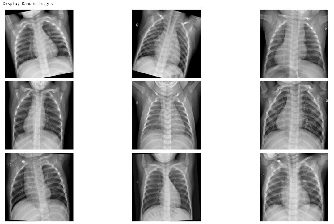
Let's visualize a few of the artificial normal images,

让我们可视化一些人工正常图像，

# Extract 9 random images
print('Display Random Images')# Adjust the size of your images
plt.figure(figsize=(20,10))for i in range(9):
    num = random.randint(0,len(n_images)-1)
    plt.subplot(3, 3, i + 1)
    
    plt.imshow(n_images[num],cmap='gray')
    plt.axis('off')
    # Adjust subplot parameters to give specified padding
plt.tight_layout()

output -

输出-

Next, let’s visualize a few of the artificial viral pneumonia images,

接下来，我们将一些人工病毒性肺炎图像可视化，

# Displays 9 generated viral images # Extract 9 random images
print('Display Random Images')# Adjust the size of your images
plt.figure(figsize=(20,10))for i in range(9):
    num = random.randint(0,len(v_images)-1)
    plt.subplot(3, 3, i + 1)
    
    plt.imshow(v_images[num],cmap='gray')
    plt.axis('off')
    # Adjust subplot parameters to give specified padding
plt.tight_layout()

output -

输出-

Each of those images generated above has some kind of augmentation — rotation, translation, flipping or blurring, all applied at random.

上面生成的那些图像中的每一个都有某种增强-旋转，平移，翻转或模糊，全部随机应用。

Next, we merge these artificial images and their labels with the original training dataset.

接下来，我们将这些人工图像及其标签与原始训练数据集合并。

new_labels = np.append(n_labels,v_labels)
y_new_labels = np.expand_dims(new_labels, axis=1)
x_new_images = np.append(n_images,v_images,axis=0)
X_train1 = np.append(X_train,x_new_images,axis=0)
y_train1 = np.append(y_train,y_new_labels)
print(X_train1.shape)
print(y_train1.shape)

output —

输出—

Now, the training dataset has 6552 images.

现在，训练数据集具有6552张图像。

bacteria_new=0
virus_new=0
normal_new =0for i in y_train1:
    
    if i==0:
        normal_new = normal_new+1
    elif i==1 :
        bacteria_new = bacteria_new+1
    else:
        virus_new=virus_new+1    
        
print ('Number of Normal images =',normal_new)
print ('Number of Bacteria images = ',bacteria_new)
print ('Number of Virus images =',virus_new)# plotting the data
xe = [i for i, _ in enumerate(labels)]
numbers = [normal_new, bacteria_new, virus_new]
plt.bar(xe,numbers,color = 'green')
plt.xlabel("Labels")
plt.ylabel("No. of images")
plt.title("Images for each label")
plt.xticks(xe, labels)
plt.show()

output —

输出—

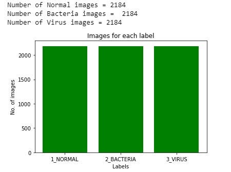
So finally, we have a balance in the training dataset. We have 2184 images in all the three classes.

因此，最后，我们在训练数据集中保持了平衡。 我们在所有三个类别中都有2184张图像。

So this is how we solved the Class Imbalance Problem. Feel free to try other methods and compare them with the final results.

因此，这就是我们解决类不平衡问题的方法。 随意尝试其他方法，并将其与最终结果进行比较。

Now that the class imbalance problem is dealt with in the next part we will look into image normalization and data augmentation using Keras and TensorFlow.

现在，在下一部分中将解决类不平衡问题，我们将研究使用Keras和TensorFlow进行图像规范化和数据增强。

翻译自: https://towardsdatascience.com/deep-learning-in-healthcare-x-ray-imaging-part-4-the-class-imbalance-problem-364eff4d47bb

x射线计算机断层成像