


 本文详细介绍了如何将TensorBoard集成到PyTorch项目中,利用其可视化功能进行深度学习模型的训练监控和超参数调优。通过实例展示了如何使用FashionMNIST数据集创建CNN模型,展示图像和图形,以及如何在训练循环中可视化评估指标。文章涵盖了从安装TensorBoard到使用其所有功能的过程,包括标量、图像和直方图的显示,以及超参数图的绘制。
In this article, we will be integrating TensorBoard into our PyTorch project. TensorBoard is a suite of web applications for inspecting and understanding your model runs and graphs. TensorBoard currently supports five visualizations: scalars, images, audio, histograms, and graphs. In this guide, we will be covering all five except audio and also learn how to use TensorBoard for efficient hyperparameter analysis and tuning.
在本文中,我们将TensorBoard集成到我们的PyTorch项目中。 TensorBoard是一套Web应用程序,用于检查和了解模型运行和图形。 TensorBoard当前支持五种可视化: 标量,图像,音频,直方图和图形 。 在本指南中,我们将涵盖除音频以外的所有五个内容,还将学习如何使用TensorBoard进行有效的超参数分析和调整。
安装指南: (Installation Guide:)
Make sure that your PyTorch version is above 1.10. For this guide, I’m using version 1.5.1. Use this command to check your PyTorch version.
确保您的PyTorch版本高于1.10。 对于本指南,我使用的是1.5.1版。 使用此命令检查您的PyTorch版本。
import torch
print(torch.__version__)
2. There are two package managers to install TensordBoard — pip or Anaconda. Depending on your python version use any of the following:
2.有两个安装TensordBoard的软件包管理器-pip 或Anaconda 。 根据您的python版本,使用以下任何一种:
Pip installation command:
点安装命令:
pip install tensorboardAnaconda Installation Command:
Anaconda安装命令:
conda install -c conda-forge tensorboardNote: Having TensorFlow installed is not a prerequisite to running TensorBoard, although it is a product of the TensorFlow ecosystem, TensorBoard by itself can be used with PyTorch.
注意:虽然安装TensorFlow不是运行TensorBoard的先决条件,尽管它是TensorFlow生态系统的产品,但TensorBoard本身可以与PyTorch一起使用。
介绍: (Introduction:)
In this guide, we will be using the FashionMNIST dataset (60,000 clothing images and 10 class labels for different clothing types) which is a popular dataset inbuilt in the torch vision library. It consists of images of clothes, shoes, accessories, etc. along with an integer label corresponding to each category. We will create a simple CNN classifier and then draw inferences from it. Nonetheless, this guide will help you extend the power of TensorBoard to any project in PyTorch that you might be working on including ones that are created using Custom Datasets.
在本指南中,我们将使用FashionMNIST数据集(60,000幅服装图像和10种针对不同服装类型的类别标签),该数据集是内置在火炬视觉库中的流行数据集。 它由衣服,鞋子,配饰等的图像以及对应于每个类别的整数标签组成。 我们将创建一个简单的CNN分类器,然后从中得出推论。 尽管如此,本指南仍将帮助您将TensorBoard的功能扩展到您可能正在从事的PyTorch项目中,包括使用自定义数据集创建的项目。
Note that in this guide we will not go into details of implementing the CNN model and setting up the training loops. Instead, the focus of the article will be on the bookkeeping aspect of Deep Learning projects to get visuals of the inner workings of the models(weights and biases) and the evaluation metrics(loss, accuracy, num_correct_predictions) along with hyperparameter tuning. If you are new to the PyTorch framework take a look at my other article on Implementing CNN in PyTorch(working with datasets, creating models and training loops) before moving forward.
请注意,在本指南中,我们将不介绍实现CNN模型和设置训练循环的详细信息。 相反,本文的重点将放在深度学习项目的簿记方面,以直观了解模型的内部工作原理(权重和偏差)和评估指标( 损失,准确性,num_correct_predictions )以及超参数调整。 如果您不熟悉PyTorch框架,请继续阅读我的另一篇有关在PyTorch中实现CNN ( 使用数据集,创建模型和训练循环 )的文章。
导入库和助手功能: (Importing Libraries and Helper Functions:)
import torch
import torch.nn as nn
import torch.optim as opt
torch.set_printoptions(linewidth=120)
import torch.nn.functional as F
import torchvision
import torchvision.transforms as transformsfrom torch.utils.tensorboard import SummaryWriter
The last command is the one which enables us to import the Tensorboard class. We will be creating instances of “SummaryWriter” and then add our model’s evaluation features like loss, the number of correct predictions, accuracy, etc. to it. One of the novel features of TensorBoard is that we simply have to feed our output tensors to it and it displays the plot of all those metrics, in this way TensorBoard can take care of all the plotting for us.
最后一个命令使我们能够导入Tensorboard类。 我们将创建“ SummaryWriter”的实例,然后向其添加模型的评估功能,例如损失,正确预测的数量,准确性等。 TensorBoard的新颖特征之一就是我们只需向其输入输出张量,并显示所有这些度量的绘图,这样TensorBoard可以为我们处理所有绘图。
def get_num_correct(preds, labels):
    return preds.argmax(dim=1).eq(labels).sum().item()
This line of code helps us to get the number of correct labels after training of the model and applying the trained model to the test set. “argmax “ gets the index corresponding to the highest value in a tensor. It’s taken across the dim=1 because dim=0 corresponds to the batch of images.”eq” compares the predicted labels to the True labels in the batch and returns 1 if matched and 0 if unmatched. Finally, we take the sum of the 1’s to get total number of correct predictions.
此代码行有助于我们在训练模型并将训练后的模型应用于测试集之后获取正确的标签数量。 “ argmax”获得与张量中最大值对应的索引。 它是在dim = 1上进行的,因为dim = 0对应于这批图像。 “ eq”将批次中的预测标签与True标签进行比较,如果匹配则返回1,如果不匹配则返回0。 最后,我们取1的总和来获得正确预测的总数。
CNN模型: (CNN Model:)
We create a simple CNN model by passing the images through two Convolution layers followed by a set of fully connected layers. Finally we will use a Softmax Layer at the end to predict the class labels.
我们通过将图像通过两个卷积层,然后是一组完全连接的层,来创建一个简单的CNN模型。 最后,我们将在最后使用Softmax层来预测类标签。
class CNN(nn.Module):
    def __init__(self):
        super().__init__()
        self.conv1 = nn.Conv2d(in_channels=1, out_channels=6, kernel_size=5)
        self.conv2 = nn.Conv2d(in_channels=6, out_channels=12, kernel_size=5)
        self.fc1 = nn.Linear(in_features=12*4*4, out_features=120)
        self.fc2 = nn.Linear(in_features=120, out_features=60)
        self.out = nn.Linear(in_features=60, out_features=10)
    def forward(self, x):
        x = F.relu(self.conv1(x))
        x = F.max_pool2d(x, kernel_size = 2, stride = 2)
        x = F.relu(self.conv2(x))
        x = F.max_pool2d(x, kernel_size = 2, stride = 2)
        x = torch.flatten(x,start_dim = 1)
        x = F.relu(self.fc1(x))
        x = F.relu(self.fc2(x))
        x = self.out(x)
        return x
导入数据并创建火车装载者: (Importing data and creating the train loader:)
train_set = torchvision.datasets.FashionMNIST(root="./data",
train = True,
 download=True,
transform=transforms.ToTensor())train_loader = torch.utils.data.DataLoader(train_set,batch_size = 100, shuffle = True)
使用TensorBoard显示图像和图形: (Displaying Images And Graphs with TensorBoard:)
tb = SummaryWriter()
model = CNN()
images, labels = next(iter(train_loader))
grid = torchvision.utils.make_grid(images)tb.add_image("images", grid)
tb.add_graph(model, images)
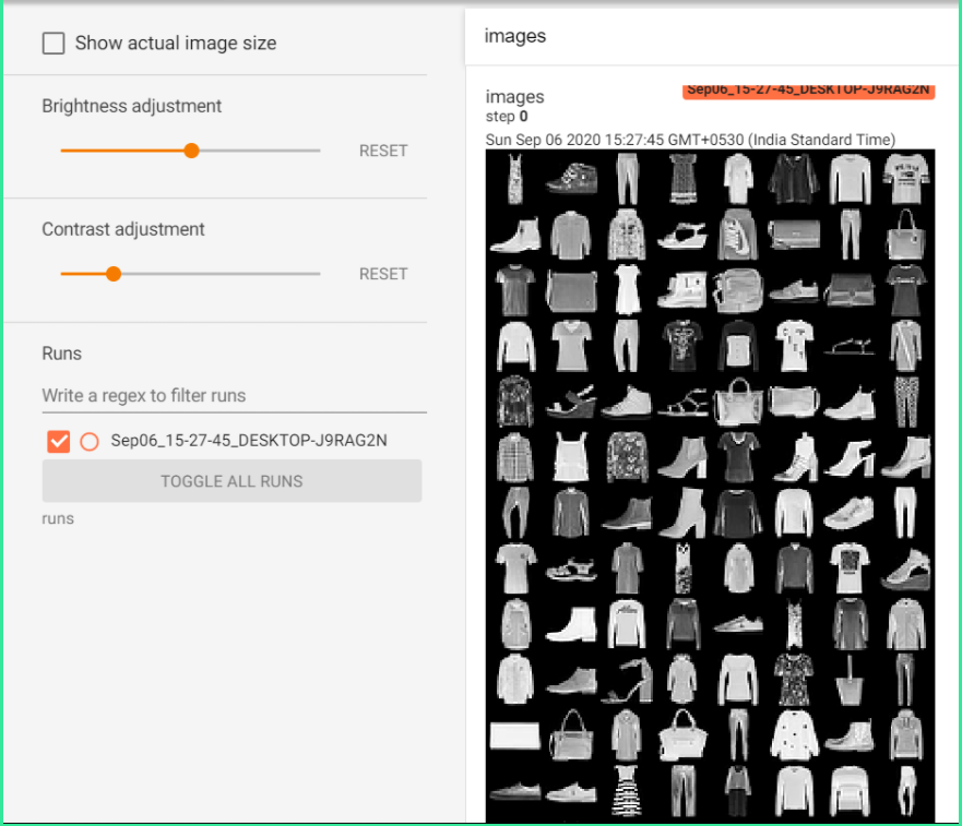
tb.close()We create an instance ‘tb’ of the SummaryWriter and add images to it by using the tb.add_image function. It takes two main arguments, one for the heading of the image and another for the tensor of images. In this case, we have created a batch of 100 images and passed them to a grid which is then added to the tb instance. To the tb.add_graph function, we pass our CNN model and a single batch of input images to generate a graph of the model. After running the code a “runs” folder will be created in the project directory. All runs going ahead will be sorted in the folder by date. This way you have an efficient log of all runs which can be viewed and compared in TensorBoard.
我们创建SummaryWriter的实例“ tb”,并使用tb.add_image函数向其添加图像。 它有两个主要参数,一个是图像的标题 ,另一个是图像的张量 。 在这种情况下,我们创建了一批100张图像,并将它们传递到网格中 ,然后将其添加到tb实例中。 向tb.add_graph函数,我们传递CNN模型和单批输入图像以生成模型图。 运行代码后,将在项目目录中创建一个“运行”文件夹。 进行的所有运行将按日期在文件夹中排序。 这样,您就可以获得所有运行的有效日志,可以在TensorBoard中进行查看和比较。
Now use the command line(I use Anaconda Prompt) to redirect into your project directory where the runs folder is present and run the following command:
现在使用命令行(我使用Anaconda Prompt)重定向到存在runs文件夹的项目目录,然后运行以下命令:
tensorboard --logdir runsIt will then server TensorBoard on the localhost, the link for which will be displayed in the terminal:
然后它将在本地主机上为TensorBoard提供服务器,其链接将显示在终端中:

After opening the link we will be able to see all our runs. The Images are visible under the “Images” tab. We can use regex to filter through the runs and tick those that we are interested in visualizing.
打开链接后,我们将能够看到我们的所有运行。 图像在“图像”选项卡下可见。 我们可以使用正则表达式筛选运行,并勾选我们希望可视化的运行。
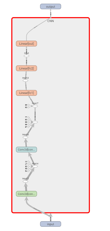
Under the “Graphs” tab you will find the graph for the model. It gives details of the entire pipeline of how the dimensions of the batch of images changes after every convolution and linear layer operations. Just double click on any of the icons to grab more information from the graph. It also gives the dimensions of all the weight and bias matrices by double-clicking on any of the Conv2d or Linear layers.
在“图形”选项卡下,您将找到模型的图形。 它提供了整个流水线的详细信息,说明在每次卷积和线性图层操作之后,图像批处理的尺寸如何变化。 只需双击任何图标即可从图形中获取更多信息。 通过双击任何Conv2d或Linear层,它也可以给出所有权重和偏差矩阵的尺寸。
训练循环以可视化评估: (Training Loop to visualize Evaluation:)
device = ("cuda" if torch.cuda.is_available() else cpu)
model = CNN().to(device)
train_loader = torch.utils.data.DataLoader(train_set,batch_size = 100, shuffle = True)
optimizer = opt.Adam(model.parameters(), lr= 0.01)
criterion = torch.nn.CrossEntropyLoss()tb = SummaryWriter()
for epoch in range(10):
total_loss = 0
total_correct = 0
for images, labels in train_loader:
images, labels = images.to(device), labels.to(device)
preds = model(images)
loss = criterion(preds, labels)
total_loss+= loss.item()
total_correct+= get_num_correct(preds, labels)
optimizer.zero_grad()
loss.backward()
optimizer.step() tb.add_scalar("Loss", total_loss, epoch)
tb.add_scalar("Correct", total_correct, epoch)
tb.add_scalar("Accuracy", total_correct/ len(train_set), epoch)
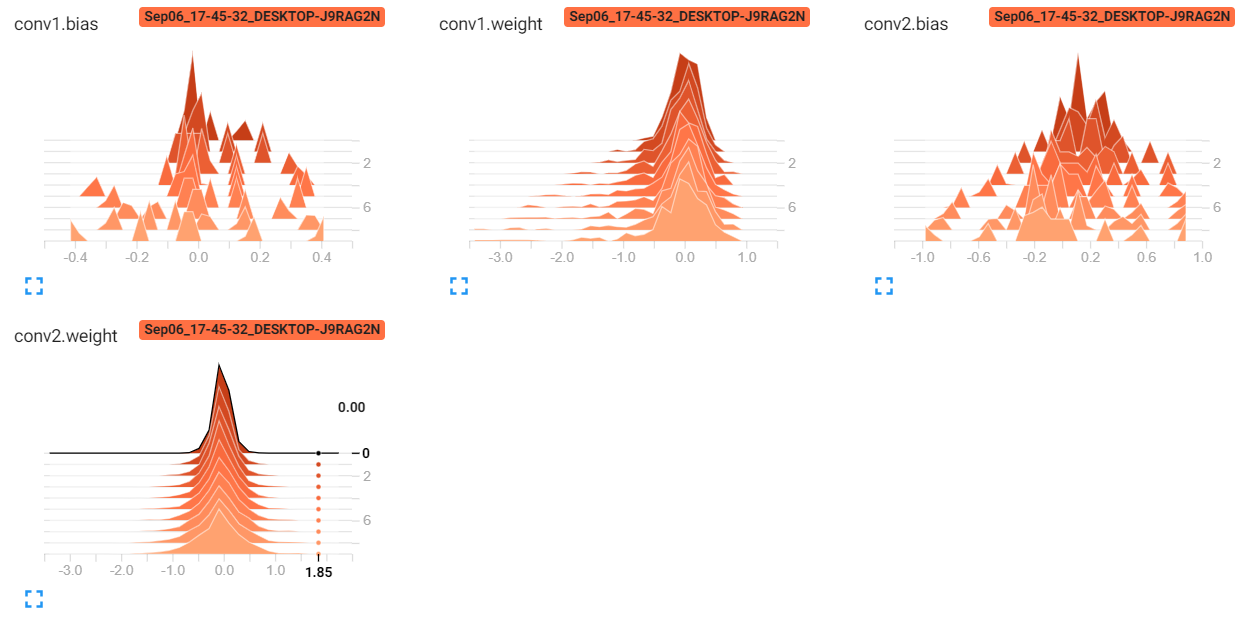
tb.add_histogram("conv1.bias", model.conv1.bias, epoch)
tb.add_histogram("conv1.weight", model.conv1.weight, epoch)
tb.add_histogram("conv2.bias", model.conv2.bias, epoch)
tb.add_histogram("conv2.weight", model.conv2.weight, epoch)
print("epoch:", epoch, "total_correct:", total_correct, "loss:",total_loss)tb.close()Alternatively, we can also use a for loop to iterate through all the model parameters including the fc and softmax layers:
另外,我们也可以使用for循环遍历所有模型参数,包括fc和softmax层:
for name, weight in model.named_parameters():    tb.add_histogram(name,weight, epoch)
    tb.add_histogram(f'{name}.grad',weight.grad, epoch)
We run the loop for 10 epochs and at the end of the training loop, we pass augments to the tb variable we created. We have created total_loss and total_correct variable to keep track of the loss and correct predictions at the end of each epoch. Note that every “tb” takes three arguments, one for the string which will be the heading of the line chart/histogram, then the tensors containing the values to be plotted, and finally a global step. Since we are doing an epoch wise analysis, we have set it to epoch. Alternatively, it can also be set to the batch id by shifting the tb commands inside the for loop for a batch by using “enumerate” and set the step to batch_id as follows:
我们将循环运行10个纪元,然后在训练循环的最后,将增量传递给我们创建的tb变量。 我们创建了total_loss和total_correct变量以跟踪损失并在每个时期结束时纠正预测 。 请注意,每个“ tb”都带有三个参数,一个用于字符串,这将是折线图/直方图的标题 ,然后是包含要绘制的值的张量,最后是一个全局步长 。 由于我们正在进行时代明智的分析,因此将其设置为时代。 另外,也可以通过使用“枚举”将for循环内的tb命令移至批处理中 ,将tb命令设置为批处理ID ,并将步骤设置为batch_id ,如下所示:
for batch_id, (images, labels) in enumerate(train_loader):
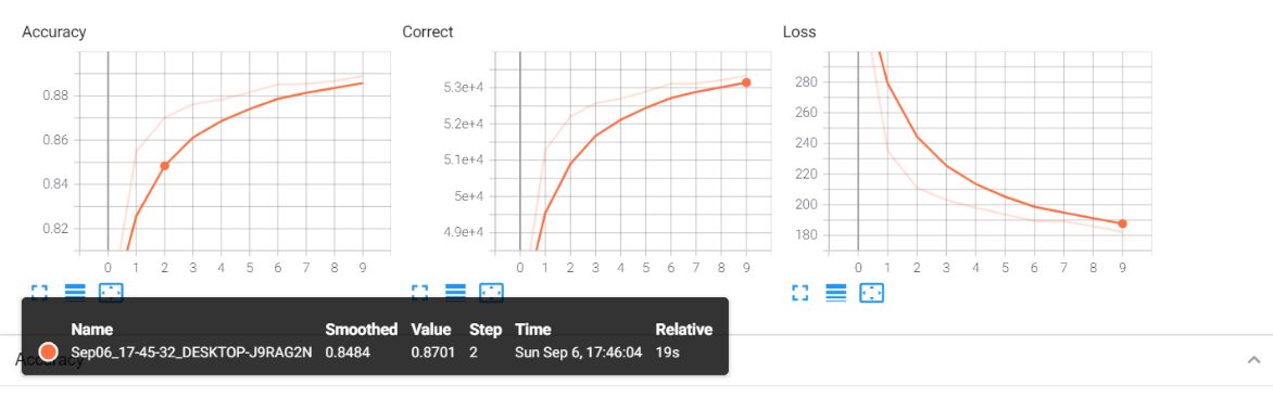
......tb.add_scalar("Loss", total_loss, batch_id)As seen below running the command mentioned earlier to run TensorBoard will display the line graph and the histograms for the loss, num_correct_predictions, and accuracy.
如下所示,运行前面提到的运行TensorBoard的命令将显示折线图和损失,num_correct_predictions和准确性的直方图。
线图: (Line Plot:)
Moving the orange dot along the graph will give us a log of the respective metric(Accuracy/Correct/Loss) for that particular epoch.
沿图形移动橙色点将为我们提供该特定时期的相应度量(准确度/正确/损失)的日志。
直方图: (Histograms:)
超参数调整: (Hyperparameter Tuning:)
Firstly we need to change the batch_size, learning_rate, shuffle to dynamic variables. We do that by creating a dictionary as follows:
首先,我们需要将batch_size,learning_rate,shuffle更改为动态变量。 为此,我们创建了一个字典,如下所示:
from itertools import product
parameters = dict(
    lr = [0.01, 0.001],
    batch_size = [32,64,128],
    shuffle = [True, False]
)
param_values = [v for v in parameters.values()]
print(param_values)
for lr,batch_size, shuffle in product(*param_values):
    print(lr, batch_size, shuffle)
This will allow us to get tuples of three, corresponding to all combinations of the three hyperparameters and then call a for loop on them before running each epoch loop. In this way, we will able to have 12 runs(2(learning_rates)*3(batch_sizes)*2(shuffles)) of all the different hyperparameter combinations and compare them on TensorBoard. We will modify the training loop as follows:
这将使我们能够获得与三个超参数的所有组合相对应的三元组,然后在运行每个时期循环之前在它们上调用for循环。 这样,我们将能够对所有不同的超参数组合进行12次运行(2(learning_rates)* 3(batch_sizes)* 2(shuffles)),并在TensorBoard上进行比较。 我们将修改训练循环,如下所示:
修改后的训练循环: (Modified Training Loop:)
for lr,batch_size, shuffle in product(*param_values):
    model = CNN().to(device)
    train_loader = torch.utils.data.DataLoader(train_set,batch_size = batch_size, shuffle = shuffle)
    optimizer = opt.Adam(model.parameters(), lr= lr)
    criterion = torch.nn.CrossEntropyLoss()comment = f' batch_size = {batch_size} lr = {lr} shuffle = {shuffle}'tb = SummaryWriter(comment=comment)
    for epoch in range(5):
        total_loss = 0
        total_correct = 0
        for images, labels in train_loader:
            images, labels = images.to(device), labels.to(device)
            preds = model(images)
            loss = criterion(preds, labels)
            total_loss+= loss.item()
            total_correct+= get_num_correct(preds, labels)
            optimizer.zero_grad()
            loss.backward()
            optimizer.step()        tb.add_scalar("Loss", total_loss, epoch)
        tb.add_scalar("Correct", total_correct, epoch)
        tb.add_scalar("Accuracy", total_correct/ len(train_set), epoch)        tb.add_hparams(
            {"lr": lr, "bsize": batch_size},
            {
                "accuracy": total_correct/ len(train_set),
                "loss": total_loss,
            },
        )
        print("batch_size:",batch_size, "lr:",lr,"shuffle:",shuffle)
        print("epoch:", epoch, "total_correct:", total_correct, "loss:",total_loss)tb.close()
As seen above we have moved everything under the for loop of to go over all different combinations of hyperparameters and at each run, we have to re-instantiate the model as well as reload the batches of the dataset. “comment” allows us to create different folders inside the runs folder depending on specified hyperparameters. We pass this comment as an argument to the SummaryWriter. Note that we will be able to see all the runs together and draw comparative analysis across all hyperparameters in TensorBoard. tb.add_scalar is the same as earlier just that we have it displayed for all runs this time. tb.add_hparams allows us to add hyperparameters inside as arguments to keep track of the training progress. It takes two dictionaries as inputs, one for the hyperparameters and another for the evaluation metrics to be analyzed. The results are mapped across all these hyperparameters. It will be clear from the graph mapping diagram at the bottom.
如上所示,我们已将for循环下的所有内容移到超参数的所有不同组合上,并且在每次运行时,我们都必须重新实例化模型并重新加载数据集的批次 。 “注释”允许我们根据指定的超参数在运行文件夹中创建不同的文件夹。 我们将此注释作为参数传递给SummaryWriter 。 请注意,我们将能够一起查看所有运行并在TensorBoard中对所有超参数进行比较分析。 tb.add_scalar与之前的相同,只是这次我们在所有运行中都显示了它。 tb.add_hparams允许我们在内部添加超参数作为自变量,以跟踪训练进度。 它使用两个字典作为输入,一个用于超参数,另一个用于待评估的评估指标。 结果映射到所有这些超参数。 从底部的图形映射图中可以清楚地看出。
组合图: (Combined Plots:)
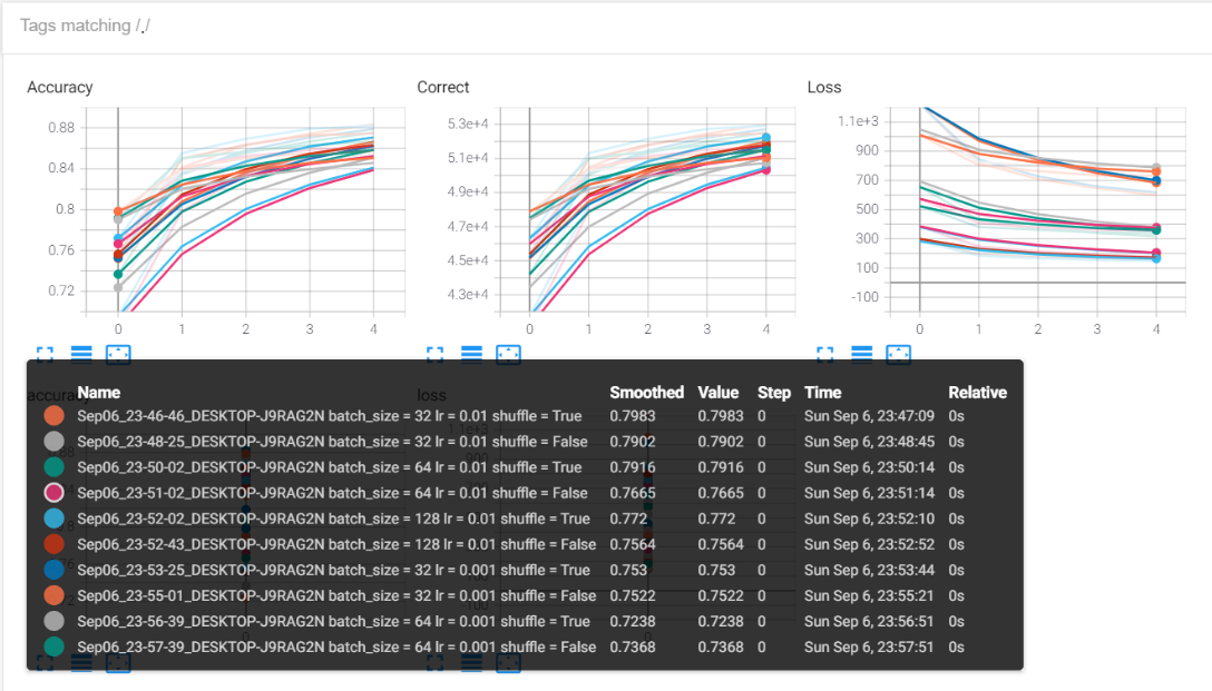
As seen above we can filter any runs that we want or have all of them plotted on the same graph. In this way, we can draw a comparative study of the performance of the model across several hyperparameters and tune the model to the ones which give us the best performance. All details like batch size, learning rate, shuffle, and corresponding accuracy values are visible in the pop-up box.
如上所示,我们可以过滤所需的任何运行或将所有运行绘制在同一张图中。 通过这种方式,我们可以对跨多个超参数的模型的性能进行比较研究,并将模型调整为能够为我们提供最佳性能的模型。 批次大小,学习率,随机播放和相应的准确性值等所有详细信息都将在弹出框中显示。
超参数图: (Hyperparameter Graph:)
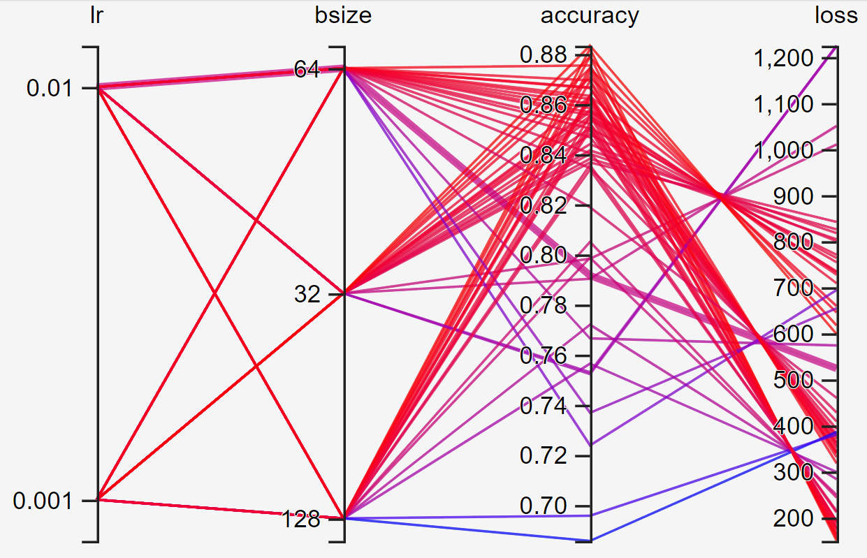
This graph has the combined logs of all 12 runs so that you can use the highest accuracy and lowest loss value and trace it back to the corresponding batch size and learning rate.
该图具有所有12次运行的组合日志,因此您可以使用最高的准确性和最低的损失值,并将其追溯到相应的批次大小和学习率。
结论: (Conclusion:)
Feel free to play around with TensorBoard, try to add more hyperparameters to the graph to gain as much information on the pattern of loss convergence and performance of the model given various hyperparameters. We could also potentially add a set of optimizers other than Adam and draw a comparative study. In cases of Sequence models like LSTMs, GRUs one can add the time-steps as well to the graph and draw insightful conclusions. Hope this article helps you feel comfortable using TensorBoard with PyTorch.
随意使用TensorBoard,尝试向图中添加更多超参数,以获取有关损耗收敛模式和给定各种超参数的模型性能的信息。 除亚当以外,我们还可能会添加一组优化器,并进行比较研究。 在诸如LSTM的序列模型的情况下,GRU可以将时间步长也添加到图形中并得出有见地的结论。 希望本文可以帮助您将TensorBoard与PyTorch结合使用。
Link to code: https://github.com/ajinkya98/TensorBoard_PyTorch
翻译自: https://towardsdatascience.com/a-complete-guide-to-using-tensorboard-with-pytorch-53cb2301e8c3


 1162
1162

 被折叠的 条评论
为什么被折叠?
被折叠的 条评论
为什么被折叠?
 到【灌水乐园】发言


