客户生命周期价值 电信行业_您的客户在整个生命中价值多少？

客户生命周期价值 电信行业

In one of my previous posts, we discussed Survival Analysis techniques to predict when our customers will churn together with customer-specific strategies to minimize customer attrition. That was in a contractual setting whereby the ‘death’ was the customer ending or not renewing their subscription.

在我以前的一篇文章中 ，我们讨论了生存分析技术以预测客户何时会流失，并结合特定于客户的策略来最大程度地减少客户流失。 那是在合同环境中，“死亡”是客户终止或不续订的。

In this post, we will look at the Buy Till You Die (BTYD) class of statistical models to analyze customers’ behavioral and purchasing patterns in a non-subscription business model to model and predict a customer’s lifetime value (CLV or LTV).

在这篇文章中，我们将研究“购买直到死亡”(BTYD)类统计模型，以在非订阅业务模型中分析客户的行为和购买模式，以建模和预测客户的生命周期价值(CLV或LTV)。

什么是客户LTV？ (What is Customer LTV?)

A customer’s Lifetime Value is the total net income or revenue that a company can expect to earn from its customers over their entire relationship — either at the individual customer level, cohort level, or over the entirety of its customer base — discounted to today’s dollar value using the Discounted Cashflow (DCF) method.

客户的生命周期价值是指公司在整个客户关系中(无论是单个客户级别，同类客户级别还是整个客户群)可以从客户那里获得的总净收入或总收入，折现成今天的美元价值使用贴现现金流量(DCF)方法。

Dependent upon what data is available, LTV can represent either total revenue or net income, i.e., revenue minus costs. It is generally less cumbersome to use revenue numbers as customer-level historical sales numbers are readily available. Whereas, the calculation of customer-specific costs might require certain assumptions, making it a bit judgemental.

根据可用的数据，LTV可以代表总收入或净收入，即收入减去成本。 使用收入数字通常比较麻烦，因为可以随时获得客户级别的历史销售数字。 鉴于客户特定成本的计算可能需要某些假设，因此有点判断力。

为什么选择LTV？ (Why LTV?)

In a non-contractual business model where there is no contract or subscription agreement between a company and its customers (e.g., e-commerce or retail), we can stop our purchases after any given transaction. Or we can come back after 12 months for a repeat purchase. Therefore, there is no distinct binary event that identifies whether a specific customer is still alive or not. This makes it practically impossible to effectively predict churn as a binary event through logistic regression or decision trees.

在非合同业务模型中，如果公司与其客户之间没有合同或订阅协议(例如，电子商务或零售)，我们可以在任何给定交易之后停止购买。 或者，我们可以在12个月后再次购买。 因此，没有可识别特定客户是否还活着的独特二进制事件。 这使得实际上不可能通过逻辑回归或决策树有效地将流失预测为二进制事件。

A better way to analyze our customers with no contractual agreement is to predict instead the monetary value that we can expect our customers to spend with us in the future together with the predicted churn probability — given their historical purchasing pattern and behavior.

在没有合同约定的情况下分析客户的一种更好的方法是，根据客户的历史购买模式和行为，预测我们可以期望客户将来在我们身上花费的货币价值以及预计的客户流失概率。

Note the difference here: we do not know at the observation end date whether a customer has churned or not. Therefore, we cannot train an algorithm to predict a datapoint (churn) that is not available to us during the model training. Instead, the churn probability will be determined through other statistical and probabilistic methods based on the purchasing history.

请注意此处的区别：在观察结束日期，我们不知道客户是否搅拌。 因此，我们无法训练算法来预测模型训练期间无法获得的数据点(客户流失)。 取而代之，将基于购买历史通过其他统计和概率方法确定流失概率。

BTYD模型简介 (Introduction to BTYD Models)

We will utilize the following two statistical and probabilistic models: Beta Geometric/Negative Binomial Distribution (BG/NBD) Model¹ and the Gamma-Gamma Model of Monetary Value² to analyze the historical customer purchasing behavioral data and pattern and to predict the future frequency and monetary value of purchases. These models have been empirically proven to be better than traditional approaches and follow the Buy Till You Die (BTYD) statistical models.

我们将利用以下两个统计和概率模型： Beta几何/负二项分布(BG / NBD)模型¹和货币价值²的Gamma-Gamma模型来分析历史客户购买行为数据和模式，并预测未来的交易频率和货币购买价值。 这些模型已经通过经验证明比传统方法更好，并且遵循“买完为止”(BTYD)统计模型。

The BG/NBD model predicts the future expected number of transactions over a pre-defined period together with the probability of a customer being alive. While the Gamma-Gamma model will tie into the BG/NBD model to predict the expected monetary value of the purchases in terms of current dollar value after discounting at a predetermined discount rate.

BG / NBD模型预测在预定义期间内未来的预期交易数量以及客户还活着的可能性。 而Gamma-Gamma模型将与BG / NBD模型结合使用，以按预定折现率折现后的当前美元价值来预测购买的预期货币价值。

Both these models are implemented in the lifetimes package of Python.

这两种模型都在Python的lifetimes包中实现。

模型假设 (Model Assumptions)

At a fundamental level, the above two models rely on the following assumptions:

从根本上讲，以上两个模型基于以下假设：

• Each customer has two coins: a ‘buy’ coin that determines its probability to make a purchase and is continuously flipped by him; and a ‘die’ coin that determines its probability to quit and never purchase again that is flipped once after every purchase

  每个客户都有两个硬币：一个“ 购买 ”硬币，用于确定其购买的可能性并不断被他抛售 ； 还有一个“ 死 ”硬币，确定其退出并不再购买的可能性， 每次购买后都会翻转一次

• While active, the number of transactions made by a customer follows a Poisson Process with a transaction rate denoted by λ (expected number of transactions in a time interval). At a simplistic level, a Poisson Process is a series of discrete events where the average time between events is known, but the exact timing of events is random. The occurrence of the next event is independent of the event before. So in our case, whether a customer makes a repeat purchase is independent of its historical buying behavior. This appears counterintuitive (a customer with multiple purchases from the same business can generally be expected to return) but has held quite well in empirical studies.
  当处于活动状态时，客户进行的交易数量遵循泊松过程，其泊车率由λ(在一个时间间隔内的预期交易数量)表示。 从简单的角度讲，泊松过程是一系列离散事件，其中事件之间的平均时间是已知的，但事件的确切时间是随机的。 下一个事件的发生与之前的事件无关。 因此，在我们的案例中，客户是否重复购物与历史购买行为无关。 这似乎是违反直觉的(通常可以预期从同一家公司进行多次购买的客户会返回)，但是在实证研究中却保持了很好的状态。
• Each customer has its buy coin (with its very own probability of head and tail)
  每个客户都有自己的购买币(拥有自己的正面和反面概率)
• Similar to the ‘buy’ coin, each customer has its own ‘die’ coin with a specific probability of being alive after each transaction
  与“购买”硬币类似，每个客户都有自己的“死”硬币，每次交易后都有特定的存活概率

• After each transaction, a customer becomes inactive with probability p, i.e., after every transaction, each customer will toss the second ‘die’ coin to determine if he makes a repeat purchase or not

  在每次交易之后，客户以概率p变为不活动状态，即，在每次交易之后，每个客户都将掷出第二个“ die”硬币，以确定他是否重复购买

• The transaction rate λ and the dropout probability p vary independently across customers and follow Gamma and Beta distributions, respectively

  交易率λ和退出概率p不同客户之间独立变化，分别遵循Gamma和Beta分布

• The monetary dollar value of a customer’s given transaction varies randomly around its average transaction value
  客户给定交易的货币美元价值在其平均交易价值附近随机变化
• Average transaction values vary across different customers but do not change over time for any given individual
  不同客户的平均交易价值各不相同，但对于任何给定的个人，其平均交易额都不会随时间变化
• The distribution of average transaction values across customers is independent of the transaction process
  客户之间平均交易价值的分布与交易过程无关

资料需求 (Data Requirements)

Both BG/NBD and Gamma-Gamma models require only the following data points at the customer level:

BG / NBD和Gamma-Gamma型号在客户级别仅需要以下数据点：

• Recency represents the age of a customer when they made their most recent purchase. This is equal to the duration between a customer’s first purchase and their latest purchase. Thus, if Ms. X made only one purchase, her recency will be 0.

  新近度代表客户最近购买商品的年龄。 这等于客户首次购买与最近购买之间的持续时间。 因此，如果X女士只购物一次，那么她的新近度将为0。

• Frequency represents the number of periods in which a customer made repeat purchases. This means that it is one less than the total number of periods in which a customer made purchases. If using days as units, then Frequency is the count of days (or whatever time period) the customer purchased after its first purchase. In case a customer made only one purchase, his Frequency will be 0. Also, frequency does not account for multiple purchases within the same time unit. Accordingly, if Mr. Y made two purchases on day 1 and three purchases on day 3, his frequency will still be 1 despite the multiple daily purchases.

  频率表示客户重复购买的期间数。 这意味着它比客户进行购买的期间总数少一个。 如果使用天为单位，则频率是客户首次购买后购买的天数(或任何时间段)。 如果客户仅进行一次购买，则其频率将为0。而且，频率不会在同一时间单位内考虑多次购买。 因此，如果Y先生在第1天进行了两次购买，在第3天进行了三次购买，则尽管每天进行多次购买，他的频率仍为1。

• Time represents the age of a customer in whatever time units are chosen. This is equal to the duration between a customer’s first purchase and the end of the period under study.

  时间代表选择任何时间单位的客户年龄。 这等于客户首次购买到研究期间结束之间的持续时间。

• Monetary Value represents the average value of a given customer’s repeat purchases, i.e., the sum of all repeat purchases divided by the total number of time units on which repeat purchases were made. Monetary value could be profit, or revenue, or any other amount as long as it is consistently calculated for each customer.

  货币价值表示给定客户重复购买的平均值，即所有重复购买的总和除以重复购买的时间单位总数。 货币价值可以是利润或收入，也可以是任何其他金额，只要为每个客户一致地计算即可。

We can extract the above four required data points from the following transaction-level data (that is usually available in internal reporting systems) through a handy utility function available in lifetimes called summary_data_from_transaction_data:

我们可以通过lifetimes可用的便捷实用工具功能(称为summary_data_from_transaction_data )从以下事务级别的数据(通常在内部报告系统中使用)中提取以上四个必需的数据点：

• Invoice or transaction date
  发票或交易日期
• invoice or transaction monetary value
  发票或交易的货币价值

BG / NBD和Gamma-Gamma模型的应用 (BG/NBD & Gamma-Gamma Models in Action)

We will use the publicly available e-commerce retail sales data for our project. This dataset contains all purchases made from an online retail company based in the UK during almost three years and can be downloaded from here.

我们将使用我们项目的公共电子商务零售数据。 该数据集包含近三年来从英国一家在线零售公司购买的所有商品，可以从此处下载。

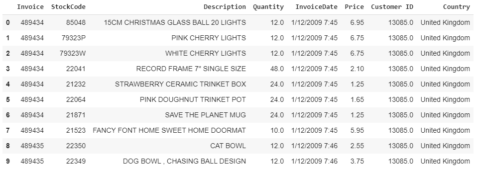
The raw data is in the following format:

原始数据采用以下格式：

数据预处理 (Data Preprocessing)

Next, we will perform the following steps to convert our raw data into the required format:

接下来，我们将执行以下步骤将原始数据转换为所需的格式：

• Convert InvoiceDate into a DateTime format and extract only the date values from it

  将InvoiceDate转换为DateTime格式，并仅从中提取日期值

• Drop rows with missing Customer ID as our analysis will be at the individual customer level

  删除缺少Customer ID行，因为我们的分析将在单个客户级别进行

• Filter out the negative values from the Quantity field as these could relate to customer returns that are not relevant to LTV predictions

  从Quantity字段中过滤出负值，因为它们可能与与LTV预测无关的客户退货有关

• Create a new column for Sales per invoice (Quantity x Price) and filter out these columns required by lifetimes: Customer ID, InvoiceDate, Sales

  为每张发票的Sales ( Quantity x Price )创建一个新列，并过滤lifetimes所需的以下列： Customer ID ， InvoiceDate ， Sales

• Transform our transaction-level data into the required summary form for lifetimes using its summary_data_from_transaction_data function

  使用其summary_data_from_transaction_data函数将我们的事务级别数据转换为lifetimes所需的摘要形式

The resultant data will be in this form:

结果数据将采用以下形式：

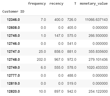
Customer # 12608 made 1 purchase only (no repeat), so both its frequency and recency are 0 as per the model definition, and its age is 405 days (i.e., the duration between the first purchase and the end of the period in the analysis). The monetary value is also 0 as it’s the mean of all the repeat purchases, thereby ignoring its only purchase.

客户＃12608仅进行了1次购买(无重复)，因此根据模型定义，其频率和新近度均为0，并且其使用期限为405天(即，从首次购买到分析期间结束之间的持续时间)。 货币价值也为0，因为它是所有重复购买的平均值，因此忽略了唯一购买。

Customer # 12745, on the other hand, made 2 purchases in total, therefore:

另一方面，客户＃12745共进行了2次购买，因此：

• frequency is 1, i.e., 1 repeat purchase

  frequency为1，即重复购买1次

• recency is the number of days between the 2 purchases

  recency是两次购买之间的天数

• T is the number of days between the first purchase and observation end date

  T是首次购买到观察结束日期之间的天数

• monetary_value is the total value of the 2nd purchase, i.e., the only repeat purchase. For more than 1 repeat purchases, it would have been the average sales value of all the repeat purchases

  monetary_value是第二次购买的总价值，即唯一的重复购买。 如果重复购买超过1次，则应为所有重复购买的平均销售额

The last preprocessing step is to exclude customers for which we have no repeat purchases, i.e., frequency is 0. Both the BG/NBD and Gamma-Gamma models focus exclusively on performing calculations on customers with repeat transactions. If we think about it, it will be quite challenging for any model to predict the probability of future transactions and monetary value for a customer that has made only one historical purchase. Otherwise, the model will predict a 100% probability of a customer being alive who had only a single purchase transaction, which is unrealistic.

最后的预处理步骤是排除没有重复购买的客户，即频率为0。BG / NBD和Gamma-Gamma模型都专门针对具有重复交易的客户进行计算。 如果我们考虑一下，对于任何模型来说，对于仅进行一次历史购买的客户而言，预测未来交易的可能性和货币价值将是非常具有挑战性的。 否则，该模型将预测只有一次购买交易的客户还活着的可能性为100％，这是不现实的。

Code for work performed so far follows:

到目前为止执行的工作代码如下：

# import and install all required libraries
import pandas as pd
import seaborn as sns
import datetime as dt
import matplotlib.pyplot as plt
import numpy as np
! pip install lifetimes==0.11.3
from lifetimes.plotting import *
from lifetimes.utils import *
from lifetimes import BetaGeoFitter
from lifetimes import GammaGammaFitter


# Load data
data = pd.read_csv('.../OnlineRetail_2yrs.csv', encoding = 'unicode_escape')


# Convert InvoiceDate into DateTime format and extract the date values
data['InvoiceDate'] = pd.to_datetime(data['InvoiceDate']).dt.date


# drop rows with missing CustomerID as our analysis will be at the individual customer level
data.dropna(axis = 0, subset = ['Customer ID'], inplace = True)


# filter out the negative values from Quantity field as these could relate to returns that are not relevant to LTV predictions
data = data[(data['Quantity'] > 0)]


# create a new column for Sales per invoice and filter out only the required columns for the Lifetimes package
data['Sales'] = data['Quantity'] * data['Price']
data_final = data[['Customer ID', 'InvoiceDate', 'Sales']]


# transform our transaction level data into the required summary form for Lifetimes
data_summary = summary_data_from_transaction_data(data_final, customer_id_col = 'Customer ID',
						  datetime_col = 'InvoiceDate', monetary_value_col = 'Sales',
						  freq = 'D')


# retain only those customers with frequency > 0
data_summary = data_summary[data_summary['frequency'] > 0]

BG / NBD模型培训和可视化 (BG/NBD Model Training & Visualisation)

Training the BG/NBD model is just like training any other ML algorithm in scikit-learn using lifetimes.BetaGeoFitter()’s fit method.

训练BG / NBD模型就像使用lifes.BetaGeoFitter lifetimes.BetaGeoFitter()的fit方法训练scikit-learn中的其他任何ML算法一样。

lifetimes has several built-in utility functions to plot and verify the BG/NBD model’s inherent assumptions:

lifetimes具有几个内置的实用程序功能，可以绘制和验证BG / NBD模型的固有假设：

• lifetimes.plotting.plot_transaction_rate_heterogeneity to plot the estimated gamma distribution of λ (customers’ propensities to purchase). Ideally, this should reflect a heterogeneous distribution, i.e., not concentrated around a single value

  lifetimes.plotting.plot_transaction_rate_heterogeneity绘制λ的估计伽马分布(客户的购买倾向)。 理想情况下，这应反映异构分布，即不集中在单个值附近

• lifetimes.plotting.plot_dropout_rate_heterogeneity to plot the estimated beta distribution of p, a customer’s probability of dropping out immediately after a transaction (the ‘die’ coin). This should also show a heterogeneous distribution

  lifetimes.plotting.plot_dropout_rate_heterogeneity绘制p的估计beta分布，即客户在交易(“硬币”)交易后立即退出的概率。 这也应显示异构分布

Although the transaction rate appears to be heterogeneous across our data, the dropout probability is less heterogeneous — most of the values are concentrated around less than 0.1 only. A potential reason could be the low number of customers with repeat purchases in our data — collecting more data over a more extended period may be beneficial for our modeling purposes. However, we will continue with our exercise and see how it goes.

尽管在我们的数据中交易速率似乎是异类的，但辍学概率却不太均匀-大多数值仅集中在小于0.1的范围内。 潜在的原因可能是我们的数据中重复购买的客户数量少-在更长的时间内收集更多数据可能对我们的建模目的有利。 但是，我们将继续进行练习，然后看看它如何进行。

模型可视化 (Model Visualizations)

Once the BG/NBD model has been trained, we can glean useful insights from the following plots:

训练完BG / NBD模型后，我们可以从以下图表中收集有用的见解：

Frequency/Recency Heatmap

频率/频率热图

This heatmap shows the number of transactions that a customer is likely to make in the next period (default is 1, i.e., next day, week, etc. based on the transaction frequency in our data), given the model parameters:

给定模型参数，此热图显示客户可能在下一个时段(根据数据中的交易频率，默认为1，即第二天，一周等)进行的下一交易次数：

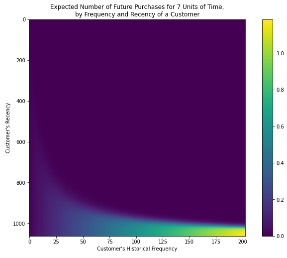
I have used T = 7 as the function’s parameter to analyze the expected number of purchases in the next 7 days.

我已使用T = 7作为函数的参数来分析未来7天的预期购买次数。

Intuitively, we can see that customers with high frequency (multiple repeat purchases) and recency (recent last repeat purchase) are expected to purchase more in the future. Our best customers are in the bottom-right of the heatmap, characterized by making more than or equal to 175 number of repeat purchases with the latest purchase being when they are more than ~1,000 days old.

凭直觉，我们可以看到频繁(多次重复购买)和新近度(最近一次重复购买)的客户将来会购买更多。 我们的最佳客户位于热图的右下角，其特征是重复购买次数超过或等于175次，而最近一次购买的时间超过了大约1000天。

In short:

简而言之：

• Customers with multiple repeat purchases (frequency) and with a higher time gap between their first and latest purchase (recency) will likely be the best customers in the future
  多次重复购买(频率)且第一次购买和最近一次购买之间的时间间隔较大(新近度)的客户可能会成为将来的最佳客户
• Customers who have made multiple repeat purchases (frequency) but with a lower time gap between their first and latest purchase (recency) (top-right corner) will probably never return
  进行过多次重复购买(频率)但第一次和最近一次购买之间的时间间隔(最近)(右上角)较小的客户可能永远不会回来
• Customers in the light blue and green zones are of interest since they may or may return for purchase, but we can still expect them to purchase about 0.7 times over the next seven days. These are the customers that may need a little cajoling or push to come back and buy more
  浅蓝色和绿色区域的客户很感兴趣，因为他们可能会或可能会再次购买，但我们仍然可以期望他们在接下来的7天内购买约0.7次。 这些客户可能需要一点儿劝说或推动才能回来购买更多产品

Probability of Alive Heatmap

存活热图的概率

This heatmap shows the probability that a customer is alive given the model parameters:

此热图显示在给定模型参数的情况下客户还活着的可能性：

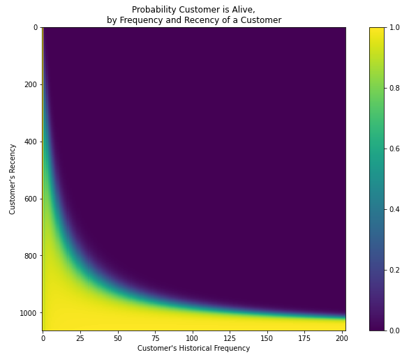
Irrespective of whether a customer purchases frequently or not, its likelihood of being alive is almost 1.0 as long as they have historically high recency (i.e., a gap of more than or equal to ~1,000 days between their first and latest purchase).

不论客户是否经常购物，只要他们的历史新高(即首次购物和最近一次购物之间的间隔大于或等于1000天)，其存活的可能性就几乎为1.0。

Also, customers with slightly lower recency (i.e., the latest purchase was after a relatively short time period from their first purchase) have a higher probability of being alive even if they do not make a high number of repeat purchases.

而且，新近度略低的客户(即，最近的购买是在第一次购买后的相对较短的时间之后)，即使他们没有进行大量重复购买，也更有可能存活。

Customers who have purchased a lot but with shorter recency are likely to have dropped out (top-right quadrant).

购买很多但新近度较短的客户可能会退出(右上象限)。

Code for model training and visualizations follows:

用于模型训练和可视化的代码如下：

# fit the BG/NBD model to our data_summary
bgf = BetaGeoFitter()
bgf.fit(data_summary['frequency'], data_summary['recency'], data_summary['T'])


# plot the estimated gamma distribution of λ (customers' propensities to purchase)
plot_transaction_rate_heterogeneity(bgf);


# plot the estimated beta distribution of p, a customers' probability of dropping out immediately after a transaction
plot_dropout_rate_heterogeneity(bgf);


# visualize our frequency/recency matrix
fig = plt.figure(figsize=(12,8))
plot_frequency_recency_matrix(bgf, T = 7);


# Now let's visualise the probability of a customer being alive
fig = plt.figure(figsize=(12,8))
plot_probability_alive_matrix(bgf);

BG / NBD模型验证 (BG/NBD Model Validation)

To perform model cross-validation, we can partition our transactional data into calibration and a holdout dataset. We will then use the holdout dataset as production data (not seen during model training), fit a new BG/NBD model on calibration data, and compare the predicted and actual number of repeat purchases over the holdout period.

为了执行模型交叉验证，我们可以将事务数据划分为校准和保留数据集。 然后，我们将使用保留数据集作为生产数据(在模型训练中看不到)，在校正数据上拟合新的BG / NBD模型，并比较保留期间重复购买的预计数量和实际数量。

A plot comparing the averages of the actual and predicted number of repeat purchases over the holdout period reveals the following:

比较保留期间内实际和预计重复购买次数的平均值的图表显示了以下内容：

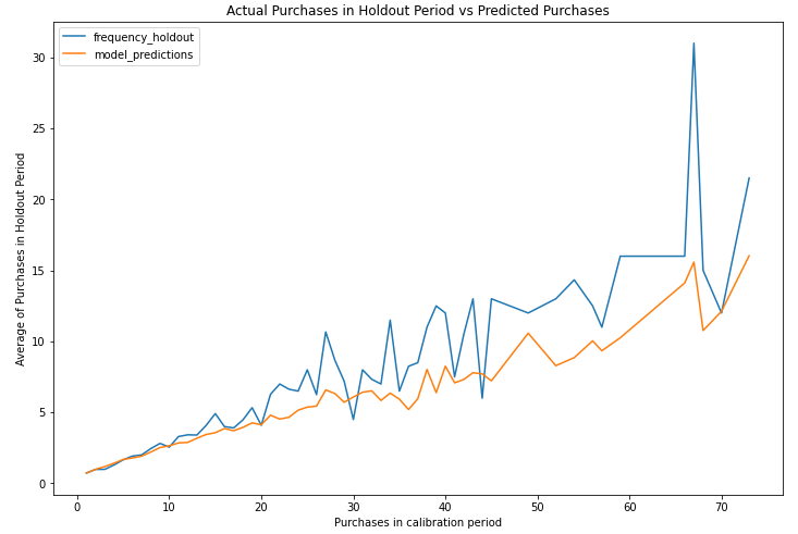
In the plot above:

在上图中：

• the x-axis represents the frequency values observed in the calibration period
  x轴表示在校准期间观察到的频率值
• the y-axis represents the average frequency in the holdout period (blue line) and the average frequency predicted by the model (orange line)
  y轴表示保留期间的平均频率(蓝线)和模型预测的平均频率(橙线)

As we can see, up to around fifteen repeat purchases, the model can very accurately predict the customer base’s behavior. For higher frequency values, the model does produce a lot more error and under-estimates the average repeat purchases. As indicated earlier, this is most likely caused by a relatively low number of customers in our data with a large number of repeat purchases.

如我们所见，该模型最多可以重复十五次，可以非常准确地预测客户群的行为。 对于较高的频率值，该模型的确会产生更多的误差，并低估了平均重复购买次数。 如前所述，这很可能是由于我们数据中的客户数量相对较少且重复购买次数较多。

Code for BG/NBD model validation:

BG / NBD模型验证代码：

# partition the dataset into a calibration and a holdout dataset
summary_cal_holdout = calibration_and_holdout_data(
	data_final, 'Customer ID', 'InvoiceDate', freq = "D", monetary_value_col = 'Sales',
	calibration_period_end='2011-06-30')


# again, retain only the +ve frequency_cal values
summary_cal_holdout = summary_cal_holdout[summary_cal_holdout['frequency_cal'] > 0]


# train BG/NBD model on the calibration data
bgf_cal = BetaGeoFitter()
bgf_cal.fit(summary_cal_holdout['frequency_cal'], summary_cal_holdout['recency_cal'],
			summary_cal_holdout['T_cal'])


# plot actual vs predicted frequency during the holdout period
plot_calibration_purchases_vs_holdout_purchases(
	bgf_cal, summary_cal_holdout, n = int(summary_cal_holdout['frequency_holdout'].max()),
	figsize = (12,8));
# n represents the max frequency values to be plotted on the x-axis

伽玛-伽玛模型训练 (Gamma-Gamma Model Training)

Now we will fit the Gamma-Gamma model on our data to calculate the probable future sales of each of our customers given their purchasing patterns.

现在，我们将在数据上拟合Gamma-Gamma模型，以根据给定的购买模式来计算每个客户的未来可能的销售额。

Can’t be easier than this:

没有比这更容易的了：

# fit the Gamma-Gamma model to our data_summary
ggf = GammaGammaFitter()
ggf.fit(frequency = data_summary['frequency'], monetary_value = data_summary['monetary_value'])

预测时间 (Prediction Time)

Now that we have our two models trained and rearing to go, let us make some predictions at the customer level. First up, we will predict the number of purchases for each customer over the next 30 days (or any other number of days of your choice):

现在我们已经训练了两个模型并进行了准备工作，让我们在客户级别进行一些预测。 首先，我们将预测接下来30天(或您选择的其他任何天数)中每个客户的购买次数：

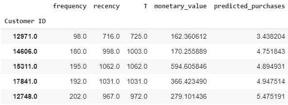
CustomerID 12748 is expected to make more between 5 and 6 purchases over the next 30 days.

客户ID 12748预计在未来30天内进行5到6次购买。

Next, we will calculate the customers’ probability of being alive and plot its distribution:

接下来，我们将计算客户存活的可能性并绘制其分布图：

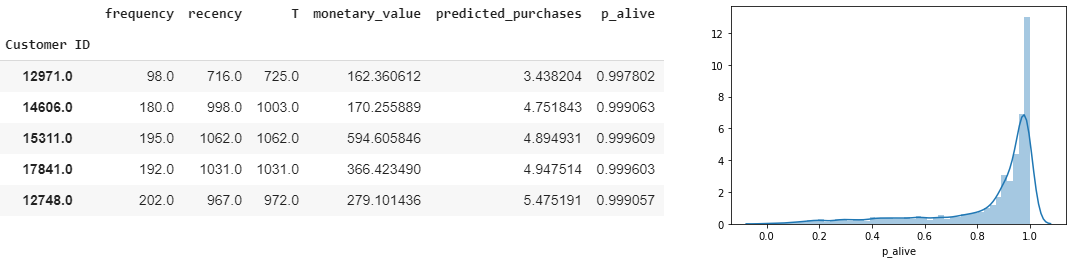
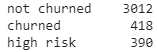
The distribution plot reveals the majority of the customers are expected to have a high possibility of being alive. After discussing with the business and marketing teams, suppose that we decide on the following probability thresholds to classify our customers:

分布图显示，预计大多数客户还活着。 与业务和营销团队讨论之后，假设我们决定以下概率阈值对客户进行分类：

• churned if the probability of being alive is less than 0.5
  如果存活的可能性小于0.5，则进行搅动
• high churn risk if the probability of being alive is between 0.5 and 0.75
  如果活着的可能性在0.5到0.75之间，则有较高的流失风险
• not churned otherwise
  否则不搅动

We get the following counts:

我们得到以下计数：

Next, we will use our trained Gamma-Gamma model to predict the average future transaction value and LTV over the next 12 months with an assumed monthly discount rate of 0.01%. Based on the expected LTV, our top 20 customers are:

接下来，我们将使用训练有素的Gamma-Gamma模型来预测未来12个月的平均未来交易价值和LTV，并假设每月贴现率为0.01％。 根据预期的LTV，我们的前20名客户是：

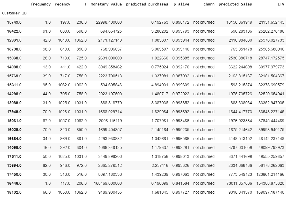
We now have our estimated churn, future purchase values, and LTVs for each of our customers who had purchased more than once with us historically.

现在，我们为每位历史上与我们进行过多次购买的客户提供了估计的客户流失率，未来的购买价值和LTV。

Code for predictions:

预测代码：

# Calculate the expected number of repeat purchases up to time t
t = 30 # to calculate the number of expected repeat purchases over the next 30 days
data_summary['predicted_purchases'] = bgf.conditional_expected_number_of_purchases_up_to_time(
	t, data_summary['frequency'], data_summary['recency'], data_summary['T'])


# Calculate probability of being currently alive and assign to each CustomerID
data_summary['p_alive'] = bgf.conditional_probability_alive(
	data_summary['frequency'], data_summary['recency'], data_summary['T'])


sns.distplot(data_summary['p_alive']);


data_summary['churn'] = ['churned' if p_alive < 0.5 else
						 'not churned' for
						 p_alive in data_summary['p_alive']]
data_summary['churn'][(data_summary['p_alive'] >= 0.5) & (data_summary['p_alive'] < 0.75)] = "high risk"
data_summary['churn'].value_counts()


# After applying Gamma-Gamma model, now we can estimate average transaction value for each customer over his/her lifetime
data_summary['predicted_Sales'] = ggf.conditional_expected_average_profit(
	data_summary['frequency'], data_summary['monetary_value'])


# calculate LTV for each customer over the next 12 months with an assumed monthly discount rate of 0.01%
data_summary['LTV'] = ggf.customer_lifetime_value(
    bgf, 
    data_summary['frequency'], data_summary['recency'], data_summary['T'], data_summary['monetary_value'],
    time = 12, # number of months to predict LTV for
    discount_rate = 0.01 # monthly discount rate ~ 12.7% annually
)


# identify our top 20 customers based on LTV
best_projected_cust_LTV = data_summary.sort_values('LTV').tail(20)
best_projected_cust_LTV

结论 (Conclusion)

Now we have some actionable insights into our most valuable and at-risk customers despite there being no contractual agreement in place with them.

现在，我们与最有价值和处于风险中的客户有了一些可行的见解，尽管他们之间没有签订合同协议。

The complete Jupyter notebook is available on GitHub here.

完整的Jupyter笔记本可在GitHub上找到 。

As always, feel free to reach out to me if you would like to discuss anything related to data analytics, machine learning, financial and credit risk analysis.

与往常一样，如果您想讨论与数据分析，机器学习，财务和信用风险分析有关的任何事情，请随时与我联系 。

Till next time, code on!

直到下一次，编码！

翻译自: https://towardsdatascience.com/what-is-your-customers-worth-over-their-lifetime-dfae277fd166

客户生命周期价值 电信行业