贷款违约预测带有真实银行数据的端到端ml项目1

表中的内容 (Table of Content)

· Introduction· About the Dataset· Import Dataset into the Database· Connect Python to MySQL Database· Feature Extraction· Feature Transformation· Modeling· Conclusion and Future Directions· About Me

· 简介 · 关于数据集 · 将数据集 导入数据库 · 将Python连接到MySQL数据库 · 特征提取 · 特征转换 · 建模 · 结论和未来方向 · 关于我

Note: If you are interested in the details beyond this post, the Berka Dataset, all the code, and notebooks can be found in my GitHub Page.

注意 ：如果您对本文之外的详细信息感兴趣，可以在我的GitHub Page中找到Berka Dataset，所有代码和笔记本。

介绍 (Introduction)

For banks, it is always an interesting and challenging problem to predict how likely a client is going to default the loan when they only have a handful of information. In the modern era, the data science teams in the banks build predictive models using machine learning. The datasets used by them are most likely to be proprietary and are usually collected internally through their daily businesses. In other words, there are not many real-world datasets that we can use if we want to work on such financial projects. Fortunately, there is an exception: the Berka Dataset.

对于银行而言，预测客户仅拥有少量信息时将拖欠贷款的可能性始终是一个有趣且具有挑战性的问题。 在现代时代，银行中的数据科学团队使用机器学习来构建预测模型。 他们使用的数据集很可能是专有数据，通常是通过日常业务在内部收集的。 换句话说，如果我们要从事此类金融项目，则可以使用的现实世界数据集并不多。 幸运的是，有一个例外： Berka Dataset 。

关于数据集 (About the Dataset)

The Berka Dataset, or the PKDD’99 Financial Dataset, is a collection of real anonymized financial information from a Czech bank, used for PKDD’99 Discovery Challenge. The dataset can be accessed from my GitHub page.

Berka数据集或PKDD'99财务数据集是来自捷克银行的真实匿名财务信息的集合，用于PKDD'99发现挑战赛。 可以从我的GitHub页面访问该数据集。

In the dataset, 8 raw files include 8 tables:

在数据集中，8个原始文件包括8个表：

• account (4500 objects in the file ACCOUNT.ASC) — each record describes static characteristics of an account.

  帐户 (文件ACCOUNT.ASC中有4500个对象)—每个记录描述一个帐户的静态特征。

• client (5369 objects in the file CLIENT.ASC) — each record describes characteristics of a client.

  客户 (文件CLIENT.ASC中有5369个对象)—每个记录都描述了客户的特征。

• disposition (5369 objects in the file DISP.ASC) — each record relates together a client with an account i.e. this relation describes the rights of clients to operate accounts.

  处置 (文件DISP.ASC中的5369个对象)—每个记录将一个客户与一个帐户关联在一起，即该关系描述了客户操作帐户的权利。

• permanent order (6471 objects in the file ORDER.ASC) — each record describes characteristics of a payment order.

  永久订单 (文件ORDER.ASC中有6471个对象)—每个记录都描述了付款订单的特征。

• transaction (1056320 objects in the file TRANS.ASC) — each record describes one transaction on an account.

  交易 (文件TRANS.ASC中有1056320个对象)—每个记录描述一个帐户上的一项交易。

• loan (682 objects in the file LOAN.ASC) — each record describes a loan granted for a given account.

  贷款 (文件LOAN.ASC中的682个对象)—每个记录都描述了为给定帐户授予的贷款。

• credit card (892 objects in the file CARD.ASC) — each record describes a credit card issued to an account.

  信用卡 (CARD.ASC文件中的892个对象)—每个记录都描述了发给帐户的信用卡。

• demographic data (77 objects in the file DISTRICT.ASC) — each record describes demographic characteristics of a district.

  人口统计数据 (文件DISTRICT.ASC中有77个对象)—每个记录都描述一个地区的人口统计特征。

Relational Dataset Repository 关系数据集存储库中的表关系

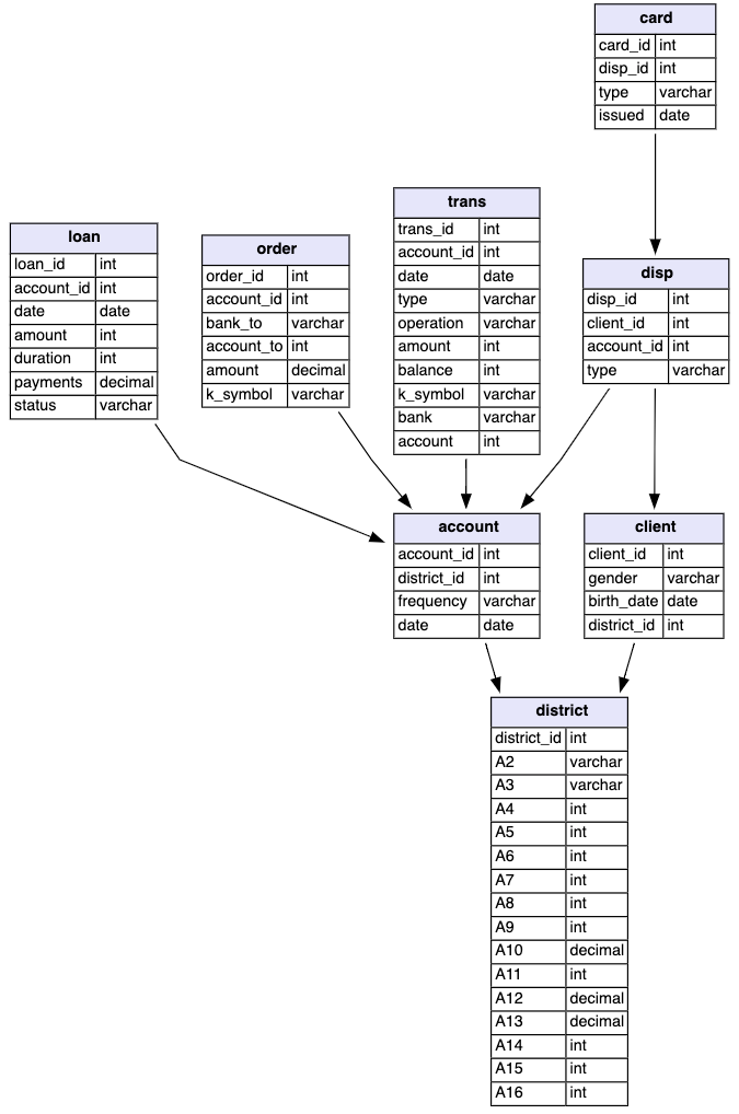
• Each account has both static characteristics (e.g. date of creation, address of the branch) given in relation “account” and dynamic characteristics (e.g. payments debited or credited, balances) given in the relations “permanent order” and “transaction”.
  每个帐户都具有在“帐户”关系中给出的静态特征(例如，创建日期，分支机构的地址)和在“永久订单”和“交易”关系中给出的动态特征(例如，借方或贷方的付款，余额)。
• Relation “client” describes the characteristics of persons who can manipulate the accounts.
  关系“客户”描述了可以操纵账户的人的特征。
• One client can have more accounts, more clients can manipulate with a single account; clients and accounts are related together in relation “disposition”.
  一个客户可以拥有更多帐户，更多的客户可以使用一个帐户进行操作； 客户和帐户在“处置”关系中相互关联。
• Relations “loan” and “credit card” describe some services which the bank offers to its clients.
  关系“贷款”和“信用卡”描述了银行向客户提供的一些服务。
• More than one credit card can be issued to an account.
  一个帐户可以发行一张以上的信用卡。
• At most one loan can be granted for an account.
  一个账户最多可以提供一笔贷款。
• Relation “demographic data” gives some publicly available information about the districts (e.g. the unemployment rate); additional information about the clients can be deduced from this.
  关系“人口数据”提供了有关地区的一些公共可用信息(例如失业率)； 由此可以推断出有关客户的其他信息。

将数据集导入数据库 (Import Dataset into the Database)

This is an optional step since the raw files contain only delimiter-separated values, so it can be directly imported into data frames using pandas.

这是一个可选步骤，因为原始文件仅包含定界符分隔的值，因此可以使用熊猫将其直接导入数据帧。

Here I wrote SQL queries to import the raw data files into MySQL database for simple and fast data manipulations (eg. select, join and aggregation functions) on the data.

在这里，我编写了SQL查询，将原始数据文件导入MySQL数据库，以便对数据进行简单，快速的数据操作(例如，选择，联接和聚合功能)。

/* Create Bank Database */
CREATE DATABASE IF NOT EXISTS bank;
USE bank;


/* Create Account Table */
CREATE TABLE IF NOT EXISTS Account(
	  account_id INT,
	district_id INT,
	frequency VARCHAR(20),
	`date` DATE
);


/* Load Data into the Account Table */
LOAD DATA LOCAL
INFILE '~/Documents/DataScience/ds_projects/loan_default_prediction/data/account.asc'
INTO TABLE Account
FIELDS TERMINATED BY ';'
ENCLOSED BY '"'
LINES TERMINATED BY '\r\n'
IGNORE 1 LINES
(account_id, district_id, frequency, @c4)
SET `date` = STR_TO_DATE(@c4, '%y%m%d');

Above is a code snippet showing how to create the bank database and import the Account table. It includes three steps:

上面的代码段显示了如何创建银行数据库和导入Account表。 它包括三个步骤：

• Create and use database
  创建和使用数据库
• Create a table
  建立表格
• Load data into the table
  将数据加载到表中

There should not be any troubles in the first two steps if you are familiar with MySQL and the database systems. For the “Load data” step, you need to make sure that you have enabled the LOCAL_INFILE in MySQL. Detailed instruction can be found from this thread.

如果您熟悉MySQL和数据库系统，则前两个步骤应该不会有任何麻烦。 对于“加载数据”步骤，您需要确保已在MySQL中启用LOCAL_INFILE 。 可以从该线程中找到详细的说明。

By repeating step 2 and step 3 on each table, all the data can be imported into the database.

通过在每个表上重复步骤2和步骤3，可以将所有数据导入数据库。

将Python连接到MySQL数据库 (Connect Python to MySQL Database)

Again, if you choose to import the data directly into Python using Pandas, this step is optional. But if you have created the database and become familiar with the dataset through some SQL data manipulations, the next step is to transfer the prepared tables into Python and perform data analysis there. One way is to use the MySQL Connector for Python to execute SQL queries in Python and make Pandas DataFrames using the results. Here is my approach:

同样，如果您选择使用Pandas将数据直接导入Python，则此步骤是可选的。 但是，如果您已创建数据库并通过一些SQL数据操作熟悉了数据集，则下一步是将准备好的表转移到Python中并在其中执行数据分析。 一种方法是使用MySQL Connector for Python在Python中执行SQL查询，并使用结果创建Pandas DataFrame。 这是我的方法：

import mysql.connector


class MysqlIO:
    """Connect to MySQL server with python and excecute SQL commands."""
    def __init__(self, database='test'):
        try:
            # Change the host, user and password as needed
            connection = mysql.connector.connect(host='localhost',
                                                 database=database,
                                                 user='Zhou',
                                                 password='jojojo',
                                                 use_pure=True
                                                 )
            if connection.is_connected():
                db_info = connection.get_server_info()
                print("Connected to MySQL Server version", db_info)
                print("Your're connected to database:", database)
                self.connection = connection
        except Exception as e:
            print("Error while connecting to MySQL", e)
            
    def execute(self, query, header=False):
        """Execute SQL commands and return retrieved queries."""
        cursor = self.connection.cursor(buffered=True)
        cursor.execute(query)
        try:
            record = cursor.fetchall()
            if header:
                header = [i[0] for i in cursor.description]
                return {'header': header, 'record': record}
            else:    
                return record
        except:
            pass
        
    def to_df(self, query):
        """Return the retrieved SQL queries into pandas dataframe."""
        res = self.execute(query, header=True)
        df = pd.DataFrame(res['record'])
        df.columns = res['header']
        return df

After modifying the database info such as host, database, user, password, we can initiate a connection instance, execute the query and convert it into Pandas DataFrame:

修改数据库信息(例如主机，数据库，用户，密码)后，我们可以启动连接实例，执行查询并将其转换为Pandas DataFrame：

# Create a connection instance
db = MysqlIO()


# Call .to_df method to execute the query and make dataframe from the results.
query = """
    select *
    from Loan join Account using(account_id);
    """
df = db.to_df(query)

Even though this is an optional step, it is advantageous in terms of speed, convenience, and good for experimentation purposes compared to directly import the files into Pandas DataFrames. Unlike other ML projects where we are only given with acsv file (1 table), this dataset is quite complicated and there is a lot of useful information hidden between the connections of tables, so this is another reason why I want to introduce the way of loading data into the database first.

即使这是一个可选步骤，与直接将文件导入Pandas DataFrames相比，它在速度，便利性和实验性方面都具有优势。 与其他仅提供csv文件(1个表)的ML项目不同，此数据集非常复杂，并且在表的连接之间隐藏了许多有用的信息，因此这也是我要介绍这种方式的另一个原因首先将数据加载到数据库中。

Now the data is in MySQL server and we have connected it Python so that we can smoothly access the data in data frames. The next steps are to extract features from the table, transform the variables, load them into one array, and train a machine learning model.

现在，数据位于MySQL服务器中，并且已将其连接到Python，以便我们可以顺利访问数据帧中的数据。 下一步是从表中提取特征，转换变量，将它们加载到一个数组中以及训练机器学习模型。

特征提取 (Feature Extraction)

Since predicting the loan default is a binary classification problem, we first need to know how many instances in each class. By looking at the status variable in the Loan table, there are 4 distinct values: A, B, C, and D.

由于预测贷款违约是一个二进制分类问题，因此我们首先需要知道每个类中有多少个实例。 通过查看“ Loan表中的status变量，有4个不同的值：A，B，C和D。

• A: Contract finished, no problems.
  答：合同完成，没有问题。
• B: Contract finished, loan not paid.
  B：合同完成，未偿还贷款。
• C: Running contract, okay so far.
  C：签合同，到目前为止还可以。
• D: Running contract, client in debt.
  D：签订合同，客户欠债。

According to the definitions from the dataset description, we can make them into binary classes: good (A or C) and bad (B or D). There are 606 loans that fall into the “good” class and 76 of them are in the “bad” class.

根据数据集描述中的定义，我们可以将它们分为二类：好(A或C)和坏(B或D)。 有606笔贷款属于“好”类，其中76笔属于“坏”类。

With the two distinct classes defined, we can look into the variables and plot the histograms to see if they correspond to different distributions.

在定义了两个不同的类之后，我们可以查看变量并绘制直方图，以查看它们是否对应于不同的分布。

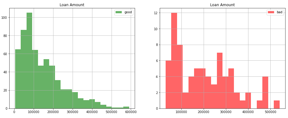
The loan amount shown below is a good example to see the difference between the two classes. Even though both are right-skewed, it still shows an interesting pattern that loans with a higher amount tend to default.

下面显示的贷款金额是了解两个类别之间差异的一个很好的例子。 即使两者都是右偏，它仍然显示出一种有趣的模式，即较高金额的贷款倾向于违约。

Histogram of Loan Amount (Good vs Bad)

贷款金额的直方图(好坏)

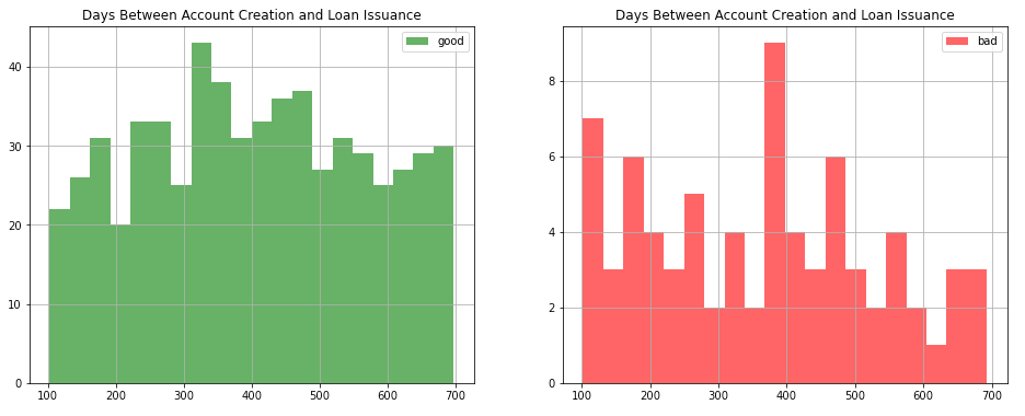
When extracting features, they don’t have to be the existing variables provided in the tables. Instead, we can always be creative and come up with some out-of-the-box solutions on creating our own features. For example, when joining the Loan table and the Account table, we can get both the date of loan issuance and the date of account creation. We may wonder if the time gap between creating the account and applying for the loan plays a role, so a simple subtraction would give us a new variable consists of days between the two such activities on the same account. The histograms are shown below, where a clear trend can be seen that people who apply for the loan right after creating the bank account tend to default.

提取要素时，它们不必是表中提供的现有变量。 相反，我们始终可以发挥创造力，并在创建我们自己的功能时提出一些现成的解决方案。 例如，当加入“ Loan表和“ Account表时，我们可以同时获得贷款发放日期和帐户创建日期。 我们可能想知道在创建帐户和申请贷款之间的时间间隔是否起作用，因此简单的减法将为我们提供一个新变量，该变量包括在同一帐户上两次此类活动之间的天数。 直方图如下所示，可以清楚地看到在创建银行帐户后立即申请贷款的人倾向于违约的趋势。

Histogram of Days between Account Creation and Loan Issuance

创建帐户与发放贷款之间的天数直方图

By repeating the process of experimenting with existing features and created features, I finally prepared a table that consists of 18 feature columns and 1 label column. The selected features are:

通过重复试验现有功能和创建的功能的过程，我最终准备了一个表，该表包含18个功能列和1个标签列。 所选功能为：

• amount: Loan amount
  金额：贷款金额
• duration: Loan duration
  期限：贷款期限
• payments: Loan payments
  付款：贷款付款
• days_between: Days between account creation and loan issuance
  days_between：创建帐户和发放贷款之间的天数
• frequency: Frequency of issuance of statements
  频率：报表的发布频率
• average_order_amount: Average amount of the permanent orders made by the account
  average_order_amount：该帐户发出的永久订单的平均数量
• average_trans_amount: Average amount of the transactions made by the account
  average_trans_amount：该帐户进行的平均交易金额
• average_trans_balance: Average balance amount after transactions made by the account
  average_trans_balance：帐户进行交易后的平均余额
• n_trans: Transaction number of account
  n_trans：帐户的交易号
• card_type: Type of credit card associated with the account
  card_type：与帐户关联的信用卡类型
• n_inhabitants: Number of inhabitants in the district of account
  n_inhabitants：帐户区域中的居民数量
• average_salary: Average salary in the district of account
  average_salary：会计区域中的平均工资
• average_unemployment: Average unemployment rate in the district of account
  average_unemployment：会计区域的平均失业率
• entrepreneur_rate: Number of entrepreneurs per 1000 inhabitants in the district of account
  企业家率：账户区每千居民中企业家人数
• average_crime_rate: Average crime rate in the district of account
  average_crime_rate：帐户区域中的平均犯罪率
• owner_gender: Account owner’s gender
  owner_gender：帐户所有者的性别
• owner_age: Account owner’s age
  owner_age：帐户所有者的年龄
• same_district: A boolean that represents if the owner has the same district information as the account
  same_district：布尔值，表示所有者是否具有与帐户相同的地区信息

特征转换 (Feature Transformation)

After the features are extracted and put into a big table, it is necessary to transform the data so that they can be fed into the machine learning model in an organic way. In our case, we have two types of features. One is numerical, such as amount, duration, and n_trans. The other one is categorical, such as card_type and owners_gender.

将特征提取并放入大表中之后，有必要对数据进行转换，以便以有机方式将其输入到机器学习模型中。 就我们而言，我们有两种类型的功能。 一个是数字 ，例如amount ， duration和n_trans 。 另一个是分类的 ，例如card_type和owners_gender 。

Our dataset is pretty clean and there is any missing value, so we can skip the imputation and directly jumpy into scaling for the numerical values. The are several options of scalers from scikit-learn , such as StandardScaler , MinMaxScaler and RobustScaler . Here, I used MinMaxScaler to rescale the numerical values between 0 and 1. On the other hand, the typical strategy of dealing with categorical variables is to use OneHotEncoder to transform the features into binary 0 and 1 values.

我们的数据集非常干净，并且没有任何遗漏的值，因此我们可以跳过插补，直接跳入数值的换算。 scikit-learn的缩放器有多个选项，例如StandardScaler ， MinMaxScaler和RobustScaler 。 在这里，我使用MinMaxScaler重新缩放0到1之间的数值。另一方面，处理分类变量的典型策略是使用OneHotEncoder将OneHotEncoder转换为二进制0和1值。

The code below is a representation of the feature transformation steps:

以下代码表示要素转换步骤：

from sklearn.compose import ColumnTransformer
from sklearn.preprocessing import OneHotEncoder, MinMaxScaler


# Define the numerical and categorical columns
num_cols = df_ml.columns[:-5]
cat_cols = df_ml.columns[-5:]


# Build the column transformer and transform the dataframe
col_trans = ColumnTransformer([
    ('num', MinMaxScaler(), num_cols),
    ('cat', OneHotEncoder(drop='if_binary'), cat_cols)
])
df_transformed = col_trans.fit_transform(df_ml)

造型 (Modeling)

The first thing in training a machine learning model is to split the train and test sets. It is tricky in our dataset because it is not balanced: there are almost 10 times more good loans than bad loans. A stratified split is a good option here because it preserves the ratio between classes in both train and test sets.

训练机器学习模型的第一件事是将训练集和测试集分开。 这在我们的数据集中非常棘手，因为它不平衡：好贷比坏贷几乎多10倍。 分层拆分在这里是一个很好的选择，因为它可以保留训练集和测试集中的类之间的比率。

from sklearn.model_selection import train_test_split


# Stratified split of the train and test set with train-test ratio of 7:3
X_train, X_test, y_train, y_test = train_test_split(X, y, test_size=0.3, 
                                            stratify=y, random_state=10)

There are many good machine learning models for binary classification tasks. Here, the Random Forest model is used in this project for its decent performance and quick-prototyping capability. An initial RandomForrestClassifier model is fit and three distinct measures are used to represent the model performance: Accuracy, F1 Score, and ROC AUC.

对于二进制分类任务，有许多好的机器学习模型。 在这里，该项目使用了随机森林模型，因为它具有不错的性能和快速原型设计能力。 初始的RandomForrestClassifier模型是拟合的，并且使用三种不同的度量来表示模型的性能： 准确性 ， F1得分和ROC AUC 。

It is noticeable that Accuracy is not sufficient for this unbalanced dataset. If we finetune the model purely by accuracy, then it would favor toward predicting the loan as “good loan”. F1 score is the harmonic mean between precision and recall, and ROC AUC is the area under the ROC curve. These two are better metrics for evaluating the model performance for unbalanced data.

值得注意的是，精度对于此不平衡数据集是不够的。 如果我们仅通过准确性对模型进行微调，那么它将有助于将贷款预测为“良好贷款”。 F1分数是精度和查全率之间的谐波平均值，ROC AUC是ROC曲线下的面积。 这两个是评估不平衡数据的模型性能的更好指标。

The code below shows how to apply 5-fold stratified cross-validation on the training set, and calculate the average of each score:

以下代码显示了如何对训练集应用5倍分层交叉验证，以及如何计算每个分数的平均值：

from sklearn.ensemble import RandomForestClassifier
from sklearn.metrics import f1_score, accuracy_score, roc_auc_score
from sklearn.model_selection import StratifiedKFold


# See the inital model performance
clf = RandomForestClassifier(random_state=10)
print('Acc:', cross_val_score(clf, X_train, y_train, 
                              cv=StratifiedKFold(n_splits=5), 
                              scoring='accuracy').mean())
print('F1:', cross_val_score(clf, X_train, y_train, 
                             cv=StratifiedKFold(n_splits=5), 
                             scoring='f1').mean())
print('ROC AUC:', cross_val_score(clf, X_train, y_train, 
                                  cv=StratifiedKFold(n_splits=5), 
                                  scoring='roc_auc').mean())

Acc: 0.8973
F1: 0.1620
ROC AUC: 0.7253

It is clearly seen that the accuracy is high, almost 0.9, but the F1 score is very low because of low recall. There is room for the model to be finetuned and strive for better performance, and one of the methods is Grid Search. By assigning different values to the hyperparameters of theRandomForestClassifier such as n_estimators max_depth min_samples_split and min_samples_leaf , it will iterate through the combinations of hyperparameters and output the one with the best performance on the score that we are interested in. A code snippet is shown below:

可以清楚地看到，准确性很高，几乎为0.9，但是由于召回率低，F1分数非常低。 可以对模型进行微调并争取更好的性能，而其中的一种方法是网格搜索。 通过向的超参数指定不同的价值RandomForestClassifier如n_estimators max_depth min_samples_split和min_samples_leaf ，它将通过超参数和输出的一个与所述分数，我们感兴趣的是一个代码段的最佳性能的组合迭代如下所示：

from sklearn.model_selection import GridSearchCV, StratifiedKFold
from sklearn.ensemble import RandomForestClassifier


# Assign different values for the hyperparameter
params = {
    'n_estimators': [10, 50, 100, 200],
    'max_depth': [None, 10, 20, 30],
    'min_samples_split': [2, 5, 10],
    'min_samples_leaf': [1, 2, 5]
}


# Grid search with 5-fold cross-validation on F1-score
clf = GridSearchCV(RandomForestClassifier(random_state=10), param_grid=params, 
                cv=StratifiedKFold(n_splits=5, shuffle=True, random_state=10),
                scoring='f1')
clf.fit(X_train, y_train)


print(clf.best_params_)

Refitting the model with the best parameters, we can take a look at the model performance one the whole train set and the test set:

用最佳参数重新拟合模型，我们可以看看整个列车和测试组的模型性能：

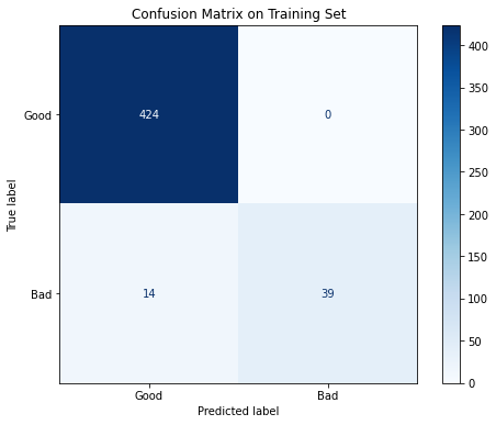
Performance on Train Set:Acc: 0.9706
F1: 0.8478
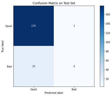
ROC AUC: 0.9952Performance on Test Set:Acc: 0.8927
F1: 0.2667
ROC AUC: 0.6957

The performance on the train set is great: more than 2/3 of the bad loans and all of the good loans are correctly classified, and all of the three performance measures are above 0.84. On the other hand, when the model is used on the test set, the result is not quite satisfying: most of the bad loans are labeled as “good” and the F1 score is only 0.267. There is evidence that overfitting is involved, so more effort should be put into such iterative processes in order to get better model performance.

火车上的表现很棒：正确分类了超过2/3的不良贷款和所有不良贷款，并且这三个绩效指标均高于0.84。 另一方面，在测试集上使用该模型时，结果并不十分令人满意：大多数不良贷款被标记为“好”，F1分数仅为0.267。 有证据表明涉及过度拟合，因此应该在这种迭代过程中付出更多的努力，以获得更好的模型性能。

With the model built, we can now rank the features based on their importance. The top 5 features that have the most prediction powers are:

建立模型后，我们现在可以根据功能的重要性对其进行排名。 具有最大预测能力的前5个功能是：

• Average Transaction Balance
  平均交易余额
• Average Transaction Amount
  平均交易金额
• Loan Amount
  贷款额度
• Average Salary
  平均工资
• Days between account creation and loan application
  创建账户和申请贷款之间的天数

There is not to much surprise here, since for many of these, we have already seen the unusual behaviors that could be related to the loan default, such as the loan amount and days between account creation and loan application.

这里并没有什么奇怪的，因为对于许多这样的情况，我们已经看到了与贷款违约有关的异常行为，例如贷款金额以及创建账户与申请贷款之间的天数 。

结论和未来方向 (Conclusion and Future Directions)

In this post, I introduced the whole pipeline of an end-to-end machine learning model in a banking application, loan default prediction, with real-world banking dataset Berka. I described the Berka dataset and the relationships between each table. Steps and codes were demonstrated on how to import the dataset into MySQL database and then connect to Python and convert processed records into Pandas DataFrame. Features were extracted and transformed into an array, ready for feeding into machine learning models. As the last step, I fit a Random Forest model using the data, evaluated the model performance, and generated the list of top 5 features that play roles in predicting loan default.

在本文中，我介绍了银行应用程序中端到端机器学习模型的整个流程，贷款违约预测以及真实银行数据集Berka。 我描述了Berka数据集以及每个表之间的关系。 演示了有关如何将数据集导入MySQL数据库，然后连接至Python并将处理后的记录转换为Pandas DataFrame的步骤和代码。 提取特征并将其转换为数组，以供输入机器学习模型。 作为最后一步，我使用数据拟合了一个随机森林模型，评估了模型的性能，并生成了在预测贷款违约中起重要作用的前5个功能的列表。

This machine learning pipeline is just a gentle touch of the one application that could be used with the Berka dataset. It could go deeper since there is more useful information hidden in the intricate relationship among tables; it could also go wider since it can be extended to other applications such as credit card and client’s transaction behaviors. But if just focusing on this loan default prediction, there could be three directions to dive further in the future:

这个机器学习管道只是可以与Berka数据集一起使用的一个应用程序的一种轻柔的接触。 由于表之间错综复杂的关系中隐藏着更多有用的信息，因此可能会更深入。 它也可以扩展，因为它可以扩展到其他应用程序，例如信用卡和客户的交易行为。 但是，如果仅关注此贷款违约预测，将来可能会有三个方向进一步跳水：

1. Extract more features: Due to the time limit, it is not possible to conduct a thorough study and have a deep understanding of the dataset. There are still many features in the dataset that are unused and a lot of the information has not been fully digested with knowledge in the banking industry.

   提取更多功能 ：由于时间限制，无法进行深入研究并深入了解数据集。 数据集中仍然有许多未使用的功能，并且银行业的知识还没有完全消化很多信息。

2. Try other models: Only the Random Forest model is used, but there are many good ones out there, such as Logistic Regression, XGBoost, SVM, or even neural networks. The models can also be improved further by finer tunings on hyperparameters or using ensemble methods such as bagging, boosting, and stacking.

   尝试其他模型 ：仅使用随机森林模型，但那里有很多好的模型，例如Logistic回归，XGBoost，SVM甚至神经网络。 还可以通过对超参数进行更精细的调整或使用集成方法(例如装袋，增强和堆叠)来进一步改进模型。

3. Deal with the unbalanced data: It is important to notice this fact that the default loans are only about 10% of the total loans, thus during the training process, the model will favor predicting more negatives than positive results. We have already used the F1 score and ROC AUC instead of just accuracy. However, the performance is still not as good as it could be. In order to solve this problem, other methods such as collecting or resampling more data can be used in the future.

   处理不平衡的数据 ：值得注意的事实是，拖欠贷款仅占总贷款的10％，因此在训练过程中，该模型将倾向于预测负数而不是正数结果。 我们已经使用了F1分数和ROC AUC，而不仅仅是准确性。 但是，性能仍未达到应有的水平。 为了解决此问题，将来可以使用其他方法，例如收集或重新采样更多数据。

关于我 (About Me)

I am a data scientist with engineering backgrounds. I embrace technology and learn new skills every day. Currently, I am seeking career opportunities in Toronto. You are welcome to reach me from Medium Blog, LinkedIn, or GitHub.

我是具有工程背景的数据科学家。 我每天都拥抱技术并学习新技能。 目前，我正在多伦多寻求职业机会。 欢迎您通过Medium Blog ， LinkedIn或GitHub与我联系 。

翻译自: https://towardsdatascience.com/loan-default-prediction-an-end-to-end-ml-project-with-real-bank-data-part-1-1405f7aecb9e