机器学习解决什么问题_机器学习帮助解决水危机

机器学习解决什么问题

According to Water.org and Lifewater International, out of 57 million people in Tanzania, 25 million do not have access to safe water. Women and children must travel each day multiple times to gather water when the safety of that water source is not even guaranteed. In 2004, 12% of all deaths in Tanzania were due to water-borne illnesses.

根据Water.org和Lifewater International的数据 ，坦桑尼亚的5700万人中，有2500万人无法获得安全的水。 妇女和儿童必须每天多次旅行以收集水，甚至不能保证该水源的安全。 2004年，坦桑尼亚所有死亡中有12％是由于水传播疾病造成的。

Despite years of effort and large amounts of funding to resolve the water crisis in Tanzania, the problem remains. The ability to predict the condition of water points in Tanzania using collectible data will allow us to build plans to efficiently utilize resources to develop a sustainable infrastructure that will affect many lives.

尽管为解决坦桑尼亚的水危机付出了多年的努力和大量资金，但问题仍然存在。 利用可收集的数据预测坦桑尼亚水位状况的能力将使我们能够制定计划，以有效利用资源来开发将影响许多生命的可持续基础设施。

数据 (Data)

As an initiative to resolve this issue, DrivenData started an exploration-based competition using data from the Tanzania Ministry of Water gathered by Taarifa, an open-source platform. The goal of the project is to predict the status of each water point in three different classes: functional, not functional and needs repair.

为了解决这个问题， DrivenData使用开放源代码平台Taarifa收集的坦桑尼亚水利部的数据，开始了基于勘探的竞赛。 该项目的目标是预测三个不同类别中每个供水点的状态：功能性，非功能性和需要维修。

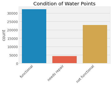
Our dataset showed that 62% of the 59,400 water points were functional while 38% were not. Out of these functional water points, 12% of them needed repairs.

我们的数据集显示，在59,400个供水点中，有62％可以正常工作，而38％则没有。 在这些功能性供水点中，有12％需要维修。

探索性数据分析 (Exploratory Data Analysis)

After cleaning the data and dealing with missing values and abnormalities, we’ve looked at how individual features may relate to the condition of water points. Here are a few observations from our exploratory data analysis.

清理数据并处理缺失值和异常之后，我们研究了各个特征如何与水位状况相关。 以下是我们探索性数据分析的一些观察结果。

不维护较旧的水位 (Older Water Points Are Not Maintained)

Here is the distribution of water points across different years of construction. We can see that most water points that are functional were built recently, which is perhaps due to the large funding that has gone in recent years. But the fact that even the ones that were built recently are as likely to be not functional as older ones is quite alarming.

这是不同施工年份的水位分布。 我们可以看到，大多数具有功能的供水点都是在最近建造的，这可能是由于近年来已投入大量资金。 但是，即使是最近制造的设备也无法像旧设备一样运行，这一事实令人震惊。

付款事宜。 (Payment Matters.)

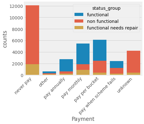
Steady payment plans seem to be a strong indicator of whether the water points would be maintained or not. The problem is that while the responsibility to maintain the water points is left to each community, most communities in Tanzania do not make enough money to upkeep these water points.

稳定的付款计划似乎是水位是否得以维持的有力指标。 问题是，维护水位的责任留给每个社区，但坦桑尼亚的大多数社区没有赚到足够的钱来养护​​这些水位。

位置事项 (Location Matters)

Based on this map of Tanzania, we can see that water point conditions tend to cluster around different areas. This tells us that location is an important predictor of this problem.

根据坦桑尼亚的这张地图，我们可以看到水位状况倾向于聚集在不同地区。 这告诉我们位置是此问题的重要预测因素。

特征工程 (Feature Engineering)

Based on our exploratory data analysis, we decided to expand on the features containing location information. First, we found the location of the basin based on its name and calculated the distance to the basin from the water points.

根据我们的探索性数据分析，我们决定扩展包含位置信息的功能。 首先，我们根据其名称找到盆地的位置，并计算出从水位到盆地的距离。

Finding the location is done using Geopy’s Nominatim package, which uses the OpenStreetMap data.

使用Geopy的Nominatim包来查找位置，该包使用OpenStreetMap数据。

from geopy.geocoders import Nominatim


def get_lat_long(location):
    # takes location string and return its longitude and latitude
    geolocator = Nominatim(user_agent = "Tanzania_water")
    location = geolocator.geocode(location)
    return (location.longitude, location.latitude)


# all unique basin from df basin column
basins = set(df.basin) 
# turn them into a dictionary
allbasins = dict.fromkeys(basins, ()) 


# for each basin, get long/lat and put in allbasins, 
# otherwise throw an error
for bas in basins:
    if allbasins[bas] != (): continue
    try:
        allbasins[bas] = get_lat_long(bas)
    except AttributeError:
        print(f"error: {bas}")

Then we calculated the distance using the geodesic distance from Geopy.

然后，我们使用距Geopy的测地线距离来计算距离。

from geopy.distance import geodesic


def get_dist(crd1, crd2): 
    # take two tuples of lat, long 
    # and return distance in miles
    return geodesic(crd1, crd2).miles


# apply it to the dataframe
df['dist_to_basin'] = df.apply(lambda x: get_dist((x.latitude, x.longitude), 
                            (x.basin_lat, x.basin_long)), axis = 1)

Also, we engineered several other features including whether the location is in the urban or rural area and the total number of other wells in the village.

此外，我们还设计了其他几个功能，包括该位置在城市还是农村地区以及该村中其他水井的总数。

前处理 (Preprocessing)

重采样 (Resampling)

Our data has a class imbalance issue, meaning that there are way more functional water points than the water points needing repairs. This can bias the prediction towards the majority class, so we used the SMOTE (synthetic minority oversampling technique) to resample our data. Simply put, SMOTE oversamples by synthesizing new samples that are close in distance to existing ones within the same class.

我们的数据存在类不平衡问题，这意味着功能上的供水点比需要维修的供水点还多。 这可能会使预测偏向多数类，因此我们使用SMOTE(合成少数过采样技术)对数据进行了重新采样。 简而言之，SMOTE通过合成与同一类别中现有样本距离最近的新样本来进行过采样。

from imblearn.over_sampling import SMOTE


smote = SMOTE() # initializing
X_train, y_train = smote.fit_sample(X_train, y_train)

In addition to resampling, we also converted the categorical features into binary dummies and standardized all features.

除了重新采样外，我们还将分类特征转换为二进制虚拟变量并标准化了所有特征。

功能选择 (Feature Selection)

Our original data had many categorical features, which resulted in a relatively large number of features after one-hot-encoding of categorical features. To optimize computation, we decided to run a tree-based feature selection.

我们的原始数据具有许多分类特征，在对分类特征进行一次热编码之后，导致了相对大量的特征。 为了优化计算，我们决定运行基于树的特征选择。

from sklearn.ensemble import ExtraTreesClassifier
from sklearn.feature_selection import SelectFromModel


# fit to a few random decision trees
etc = ExtraTreesClassifier(n_estimators=100, class_weight='balanced', n_jobs=-1)
etc = etc.fit(X_train, y_train)
# select ones with feature importance less than 0.0001
model = SelectFromModel(etc, prefit=True, threshold = 1e-4)
# tranform the data
X_train_new = model.transform(X_train)
# return the list of new features
new_feats = original_feats[model.get_support()]

模型评估 (Model Evaluation)

评估指标 (Evaluation Metrics)

Deciding on the evaluation metrics that align with the project goal is very important (if you need a refresher, see HERE). We approached this problem with two primary purposes, one is to build a model with the highest overall accuracy and another is to build a model that successfully predicts the needs repair cases. The latter was important because predicting the needs repair cases accurately is directly related to changes that affect many people’s lives in Tanzania. But for this post, I will evaluate models in terms of overall accuracy.

确定与项目目标保持一致的评估指标非常重要(如果需要复习，请参阅此处 )。 我们通过两个主要目的解决了这个问题，一个目的是建立具有最高总体准确性的模型，另一个目的是建立一个能够成功预测需求修复案例的模型。 后者之所以重要，是因为准确预测需求修复案例与影响坦桑尼亚许多人生活的变化直接相关。 但是对于这篇文章，我将根据整体准确性评估模型。

虚拟分类器 (Dummy Classifier)

First, we started by fitting a dummy classifier as our baseline model. Our dummy classifier used the stratified approach, meaning it made predictions based on the proportion of each class.

首先，我们首先将虚拟分类器拟合为基线模型。 我们的虚拟分类器使用分层方法，这意味着它根据每个类的比例进行预测。

from sklearn.metrics import accuracy_score
from sklearn.dummy import DummyClassifier


# dummy using the default stratified strategy
dummyc = DummyClassifier(strategy = 'stratified') 
dummyc.fit(X_train, y_train)
y_pred = dummyc.predict(X_test)


# report scores! 
def scoring (y_test, y_pred):
    accuracy = round(accuracy_score(y_test, y_pred), 3)
    print('Accuracy: ', accuracy)


scoring(y_test, y_pred)

Please note that the X_test in this code refers to our validation set. We have set aside the holdout set to test the final model at the end.

请注意，此代码中的X_test是指我们的验证集。 我们预留了保留集，以在最后测试最终模型。

# Dummy result: Accuracy:  0.33

Our dummy showed approximately 33% accuracy, which is an expected performance of a dummy for classifying three classes.

我们的假人显示出约33％的准确性，这是假人对三类进行分类的预期性能。

K最近邻居 (K-Nearest Neighbors)

The first model we tested was the K-Nearest Neighbors (KNN). The KNN classifies based on the classes of the k number of closest observations. The hyperparameter tuning was achieved by the Optuna. We tested the performance of both GridSearchCV and Optuna and found Optuna to be much more versatile and efficient.

我们测试的第一个模型是K最近邻居(KNN)。 KNN基于k个最接近的观测值的类别进行分类。 超参数调整是通过Optuna实现的。 我们测试了GridSearchCV和Optuna的性能，发现Optuna更具通用性和效率。

from sklearn.neighbors import KNeighborsClassifier
import optuna
from sklearn.model_selection import KFold
from sklearn.model_selection import cross_val_score


def find_hyperp_KNN(trial):
    ## Setting parameter 
    n_neighbors = trial.suggest_int('n_neighbors', 1, 31)
    algorithm = trial.suggest_categorical('algorithm', ['ball_tree', 'kd_tree'])
    p = trial.suggest_categorical('p', [1, 2])
    
    ## initialize the model
    knc = KNeighborsClassifier(weights = 'distance', 
                             n_neighbors = n_neighbors, 
                             algorithm = algorithm, 
                             p = p)
    ## assigning K-fold cross validation
    cv = KFold(n_splits = 5, shuffle = True, random_state = 20)
    
    ## calculate the average accuracy score on 5-folds cross validations
    score = np.mean(cross_val_score(knc, X_train, y_train, scoring = 'accuracy', cv = cv, n_jobs = -1))
    return (score)


# initiating the optuna study, maximize accuracy
knn_study = optuna.create_study(direction='maximize')


# run optimization for 100 trials
knn_study.optimize(find_hyperp_KNN, n_trials = 100) # use timeout to set the timer


# Testing the best params on the test set
knc_opt = KNeighborsClassifier(**knn_study.best_params)
knc_opt.fit(X_train, y_train)
y_pred = knc_opt.predict(X_test)
scoring(y_test, y_pred)

# KNN Result - Accuracy: 0.752

随机森林分类器 (Random Forest Classifier)

Next, we tested the random forest classifier with Optuna hyper-tuning. The random forest simultaneously fits multiple decision trees on a subset of the data then aggregates the results.

接下来，我们使用Optuna超调测试了随机森林分类器。 随机森林同时将多个决策树适合数据的子集，然后汇总结果。

from sklearn.ensemble import RandomForestClassifier


def find_hyperparam_rf(trial):
    ### Setting hyperparameter options ###
    n_estimators = trial.suggest_int('n_estimators', 100, 700)
    min_samples_split = trial.suggest_int('min_samples_split', 2, 10)
    min_samples_leaf = trial.suggest_int('min_samples_leaf', 1, 10)
    criterion = trial.suggest_categorical('criterion', ['gini', 'entropy'])
    class_weight = trial.suggest_categorical('class_weight', ['balanced', 'balanced_subsample'])
    max_features = trial.suggest_int('max_features', 2, X_train.shape[1]) # consider using float instead
    min_weight_fraction_leaf = trial.suggest_loguniform('min_weight_fraction_leaf', 1e-7, 0.1)
    max_leaf_nodes = trial.suggest_int('max_leaf_nodes', 10, 200)
    ### Initializing
    rfc = RandomForestClassifier(oob_score = True, 
                                 n_estimators = n_estimators,
                                 min_samples_split = min_samples_split,
                                 min_samples_leaf = min_samples_leaf,
                                 criterion = criterion,
                                 class_weight = class_weight, 
                                 max_features = max_features,
                                 min_weight_fraction_leaf=min_weight_fraction_leaf, 
                                 max_leaf_nodes = max_leaf_nodes
                                )
    ### Setting KFolds Crossvalidation
    cv = KFold(n_splits = 5, shuffle = True, random_state = 20)
    ### get the average accuracy score of 5 folds
    score = np.mean(cross_val_score(rfc, X_train, y_train,
                                    scoring = 'accuracy', cv = cv, n_jobs = -1))
    return (score)


# initialize the study
rfc_study = optuna.create_study(direction='maximize')
# run it for 3 hours or for 100 trials
rfc_study.optimize(find_hyperparam_rf, timeout = 3*60*60, n_trials = 100)


# fit the model
rf = RandomForestClassifier(oob_score = True, **rfc_study.best_params)
rf.fit(X_train, y_train)
y_pred_rf = rf.predict(X_test)
scoring(y_test, y_pred_rf)

# Random Forest Results - Accuracy : 0.74

The performance of KNN was better than the random forest classifier for this problem. But even though not reported here, the random forest classifier did a much better job at classifying the minority class than the KNN.

对于该问题，KNN的性能优于随机森林分类器。 但是，尽管这里没有报告，但随机森林分类器在分类少数族群方面比KNN的工作要好得多。

XGBoost (XGBoost)

Since we tested a bagging method, we also tried a boosting method, using the XGBoost. It’s an implementation of a gradient boosting model, which iteratively trains the weak learners based on the prediction errors it makes.

由于我们测试了装袋方法，因此我们也尝试了使用XGBoost的加强方法。 它是梯度提升模型的实现，该模型根据其产生的预测误差迭代地训练弱学习者。

import xgboost as xgb


def find_hyperparam(trial):
    ### Setting hyperparameter range ###
    eta = trial.suggest_loguniform('eta', 0.001, 1)
    max_depth = trial.suggest_int('max_depth', 1, 50)
    subsample = trial.suggest_loguniform('subsample', 0.4, 1.0)
    colsample_bytree = trial.suggest_loguniform('colsample_bytree', 0.01, 1.0)
    colsample_bylevel = trial.suggest_loguniform('colsample_bylevel', 0.01, 1.0)
    colsample_bynode = trial.suggest_loguniform('colsample_bynode', 0.01, 1.0)


    # Initializing the model
    xgbc = xgb.XGBClassifier(objective = 'multi:softmax', 
                             eta = eta, 
                             max_depth = max_depth, 
                             subsample = subsample, 
                             colsample_bytree = colsample_bytree, 
                             colsample_bynode = colsample_bynode, 
                             colsample_bylevel = colsample_bylevel)
    
    # Setting up k-fold crossvalidation
    cv = KFold(n_splits = 5, shuffle = True, random_state = 20)
    # evaluate using accuracy
    score = np.mean(cross_val_score(xgbc, X_train, y_train, 
                                    scoring = 'accuracy', cv = cv, 
                                    n_jobs = -1))
    return (score)


# initializing optuna study
xgb_study = optuna.create_study(direction='maximize')
# run optimization for 3 hours or for 100 trials
xgb_study.optimize(find_hyperparam, timeout = 3*60*60, n_trials = 100)


# testing on the test set
xgbc = xgb.XGBClassifier(**xgb_study.best_params, verbosity=1, tree_method = 'gpu_hist')
xgbc.fit(X_train, y_train)
y_pred = xgbc.predict(X_test)    
scoring(y_test, y_pred, 'xgboost')

# XGBoost Results - Accuracy: 0.78

XGboost showed improvement in the accuracy score, and its sensitivity in predicting minority class was also higher than the other two models.

XGboost的准确性得分有所提高，并且其预测少数族裔类别的敏感性也高于其他两个模型。

投票分类器 (Voting Classifier)

Lastly, we took all the previous models and put them to vote. When using a voting classifier, we can either combine each model’s prediction on the probability of each class (soft) or use its binary choice of each class (hard). Here, we used soft voting.

最后，我们采用了所有以前的模型并将它们投票。 使用投票分类器时，我们可以结合每个模型对每个类别的概率的预测(软)，也可以使用其对每个类别的二进制选择(困难)。 在这里，我们使用了软投票。

from sklearn.ensemble import VotingClassifier


voting_c_soft = VotingClassifier(estimators = [
                                          ('knc_opt', knc_opt),
                                          ('rf', rf),
                                          ('xgbc', xgbc)
                                         ], 
                            voting = 'soft', n_jobs = -1)
# fit on training, test on testing set
voting_c_soft.fit(X_train, y_train)
y_pred = voting_c_soft.predict(X_test)    
scoring(y_test, y_pred, 'voting')

# Voting Classifier - Accuracy: 0.79

Voting classifier returns slightly higher accuracy and similar recall for the minority class. We decided to continue with the voting classifier as our final model and test the holdout test set.

投票分类器返回的准确性略高，而少数民族分类的召回率相似。 我们决定继续使用投票分类器作为最终模型，并测试保留测试集。

最终模型表现 (Final Model Performance)

Our final model showed 80% prediction accuracy on the holdout set (baseline 45%), and close to 50% recall on the minority class, which is a significant improvement from 6% recall by the baseline model.

我们的最终模型在保留集上具有80％的预测准确度 (基线45％)，而在少数群体上的召回率接近50％，与基线模型的6％召回率相比有显着改善。

Photo by ngozi Assata on Unsplash

由 ngozi Assata 摄于 Unsplash

奖金：口译 (Bonus: Interpretation)

Because our final model involved voting between a distance algorithm and tree-based ensembles, it’s difficult to interpret the feature importance of our model. But additional analysis using a logic regression with the Elastic Net regularization and SGD training showed that enough quantity of water, use of communal standpipes, and being recently built were the important predictors of the functional water points.

由于我们的最终模型涉及距离算法和基于树的集成体之间的投票，因此很难解释模型的特征重要性。 但是，使用带有Elastic Net正则化和SGD训练的逻辑回归进行的其他分析表明，充足的水量，公用竖管的使用和近期兴建的水是功能性水位的重要预测指标。

On the other hand, the location was an important predictor of non-functional water points. Especially some of the northern regions closer to Lake Victoria were highly related to the non-functioning water points. Lastly, GPS heights of water point showed different patterns between the non-functional and ones that need repair. Further investigation is necessary to find the significance of GPS heights whether it’s related to the specific government area, or the difference in accessibility, or whether it has any technical implication to some of the extraction types.

另一方面，该位置是非功能水位的重要预测指标。 尤其是靠近维多利亚湖的一些北部地区与无法正常工作的水位高度相关。 最后，GPS的水位高度在非功能性和需要修复的位置之间显示出不同的模式。 无论是与特定的政府区域有关，还是在可达性方面的差异，或者对某些提取类型有任何技术影响，都必须进行进一步的调查来确定GPS高度的重要性。

This project was done in collaboration with my colleague dolcikey.

这个项目是与我的同事dolcikey合作完成的。

翻译自: https://towardsdatascience.com/machine-learning-to-help-water-crisis-24f40b628531

机器学习解决什么问题