张量图像处理_使用初学者的迁移学习进行张量流图像分类

张量图像处理

Training a machine learning model could be quite time-consuming. Especially if you are trying to solve a complex problem. One solution to speed up the training process is to use a pre-trained model. This is called transfer learning.

完善机器学习模型可能会非常耗时。 特别是如果您要解决一个复杂的问题。 加快训练过程的一种解决方案是使用预先训练的模型。 这称为转移学习。

Transfer learning allows us to use a pre-trained model to solve our problem. There are many pre-trained models out there like mobilenet, VGG, Resnet, etc. In this article, we will implement image classification using transfer learning in TensorFlow.

转移学习使我们能够使用预先训练的模型来解决我们的问题。 那里有许多预先训练的模型，例如mobilenet，VGG，Resnet等。在本文中，我们将使用TensorFlow中的转移学习来实现图像分类。

The code for this article can be found in my GitHub.

可以在我的GitHub中找到本文的代码。

First, let us import certain libraries that we are going to need while also loading our dataset. We will use TensorFlow ‘horses_or_humans’ dataset to classify whether an image is a horse or a human. We will also visualize our data.

首先，让我们导入需要的某些库，同时还要加载数据集。 我们将使用TensorFlow'horses_or_humans'数据集对图像是马还是人进行分类。 我们还将可视化我们的数据。

# import libraries
import numpy as np
import matplotlib.pyplot as plt
import tensorflow as tf
import tensorflow_datasets as tfds


# load dataset
dataset = tfds.load('horses_or_humans', split=['train'], as_supervised=True)


# take the images and the target
array = np.vstack(tfds.as_numpy(dataset[0]))
X = np.array(list(map(lambda x: x[0], array)))
y = np.array(list(map(lambda x: x[1], array)))


# visualize
f, (ax1, ax2, ax3) = plt.subplots(1, 3, figsize=(15,15))
ax1.imshow(X[0])
ax2.imshow(X[50])
ax3.imshow(X[100])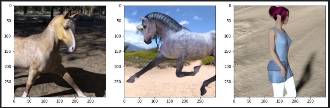

TensorFlow ‘horses_or_humans’ consists of 1027 images of horses and humans

TensorFlow'horses_or_humans'由1027张马和人类的图像组成

Next, we need to split our dataset into training and testing data. We also need to reshape our training and testing data so it matches our model.

接下来，我们需要将数据集分为训练和测试数据。 我们还需要重塑我们的训练和测试数据，使其与我们的模型相匹配。

TensorFlow provides many pre-trained models for us to play with. In this article, The pre-trained model we are going to use is ResNet50, short for Residual Networks with 50 layers. It is based on the ResNet model that won ImageNet challenge in 2015. Do not forget to set all of the ResNet50 layers un-trainable so it will not update its weight based on our training.

TensorFlow提供了许多预训练的模型供我们使用。 在本文中，我们将使用的预训练模型是ResNet50，它是具有50层的残差网络的缩写。 它基于ResNet模型，该模型在2015年赢得了ImageNet挑战。不要忘记将所有ResNet50图层设置为不可训练，因此不会根据我们的训练来更新其权重。

# split the dataset into training and testing data
from sklearn.model_selection import train_test_split


X_train, X_test, y_train, y_test = train_test_split(X, y, test_size=0.33, random_state=133, shuffle=True)


y_train = y_train.reshape(len(y_train), 1)
y_test = y_test.reshape(len(y_test), 1)


# import the Resnet50 and others libraries 
from tensorflow.keras.applications.resnet50 import ResNet50
from tensorflow.keras.models import Model, Sequential
from tensorflow.keras.layers import Dense, Flatten


# define the ResNet50
restnet = ResNet50(include_top=False, weights='imagenet', input_shape=(300,300,3))


# set all nodes on our pre-trained model to be untrainable node
# so that it will not change when we perform our own training
for layer in restnet.layers:
    layer.trainable = False


# create the model
model = Sequential()
model.add(restnet)
model.add(Flatten())
model.add(Dense(16, activation='relu', input_dim=(300,300,3)))
model.add(Dense(1, activation='sigmoid'))


# compile the model
model.compile(optimizer='Adam', loss='binary_crossentropy', metrics=['accuracy'])


model.summary()

Then, let’s train our model and also visualize its performances.

然后，让我们训练模型并可视化其性能。

# train our model
history = model.fit(
    x=X_train,
    y=y_train,
    epochs=5,
    verbose=1,
    validation_data=(X_test, y_test),
)


# visualize our training
plt.figure()
plt.plot(range(5), history.history['loss'])
plt.plot(range(5), history.history['val_loss'])
plt.ylabel('Loss')
plt.legend(['training','validation'])


# predict our data
predict = model.predict(X_test)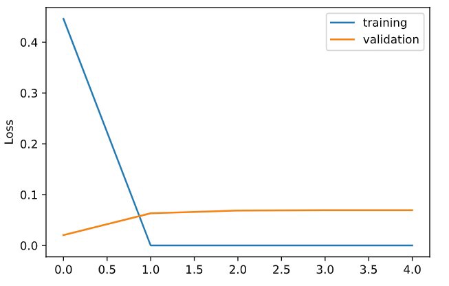

Our model performances

我们的模特表演

Let us use the testing data to see our model predictions.

让我们使用测试数据来查看模型预测。

print('Note: 0 is horse and 1 is human\n')


labels = ['horse', 'human']
f, (ax1, ax2) = plt.subplots(1, 2, figsize=(15,15))
ax1.imshow(X_test[50])
ax1.set_title("It's a " + labels[int((predict[50]))])
ax2.imshow(X_test[100])
ax2.set_title("It's a " + labels[int((predict[100]))])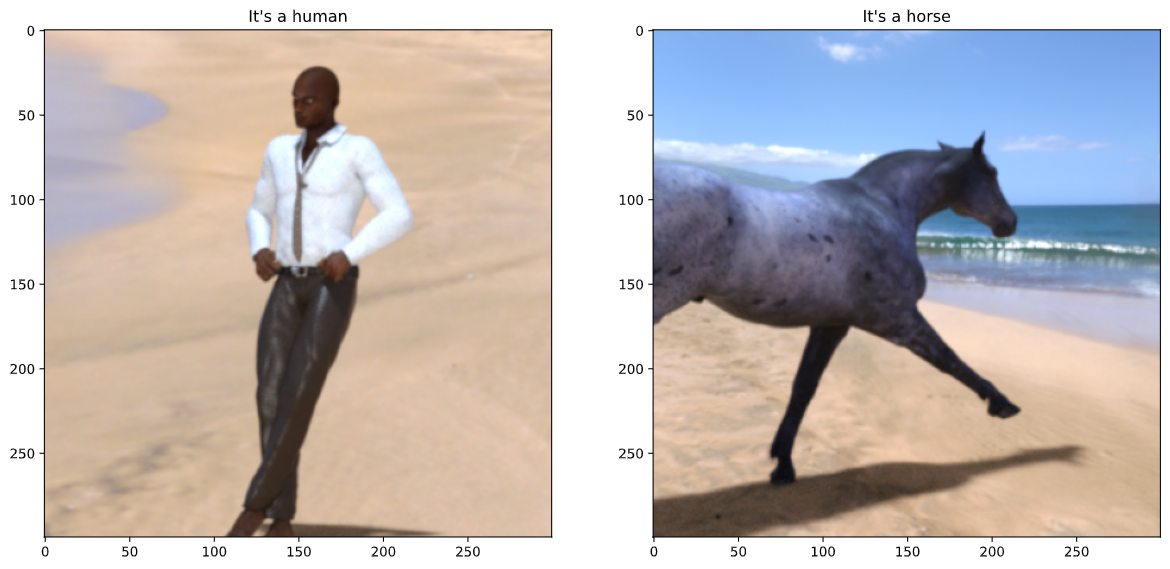

The model successfully predict the test data

该模型成功预测了测试数据

As we can see, the model successfully predicts our test data. But what about an unseen one? Can it still predict the image? Let us see.

如我们所见，该模型成功预测了我们的测试数据。 但是一个看不见的呢？ 它还能预测图像吗？ 让我们看看。

from PIL import Image


image = np.array(Image.open('horse.jfif').resize((300,300)))
plt.imshow(image)
image = image.reshape(1, 300, 300, 3)
plt.title("It's a " + labels[int(model.predict(image))])
plt.show()

The model successfully predict an unseen image

该模型成功预测了看不见的图像

翻译自: https://medium.com/the-innovation/tensorflow-image-classification-using-transfer-learning-for-beginners-e1bd94ccfcca

张量图像处理