交叉熵 kl 条件熵_交叉熵和kl发散

交叉熵 kl 条件熵

熵 (Entropy)

KL divergence has its origin in information theory. But before understanding it we need to understand another important metric in information theory called Entropy. Since this article is not about entropy I will not cover it in depth here. I wrote about it in detail here.

K L散度起源于信息论。 但是在理解它之前，我们需要了解信息论中的另一个重要指标，即熵 。 由于本文不是关于熵的，因此在此不做深入介绍。 我在这里详细介绍了它。

The main goal of information theory is to quantify how much information is in the data. Those events that are rare (low probability) are more surprising and therefore have more information than those events that are common (high probability). For example, Would you be surprised if I told you the coin with head on both sides gave head as an outcome? No, because outcomes did not give you any further information. Now if I flip a fair coin instead of biased like head on both sides, each toss gives you the new information.

信息论的主要目标是量化数据中有多少信息。 那些罕见的事件(低概率)比那些常见的事件(高概率)更令人惊讶，因此具有更多的信息。 例如，如果我告诉你两面都正面朝上的硬币以正面朝下的结果，你会感到惊讶吗？ 不可以，因为结果没有给您任何进一步的信息。 现在，如果我抛一个公平的硬币，而不是像两边的头一样偏斜，那么每次抛掷都会为您提供新的信息。

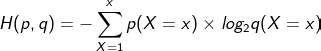
Entropy is the average amount of information conveyed by identifying the outcome of some random source. It is simply the sum of several terms, each of which is the information of a given event weighted by the probability of that event occurring. The entropy of a discrete random variable X with distribution p denoted by H(p) is defined by:

Ëntropy是信息的平均量传送通过识别一些随机源的结果。 它只是几项的总和，每一项都是给定事件的信息，由该事件发生的概率加权。 由H(p)表示的分布p的离散随机变量X的熵定义为：

Equation 1 等式1

Kullback-Leibler(KL)发散 (Kullback-Leibler (KL) Divergence)

Very often in Machine learning, we have to compare the real distribution of data with a distribution that our model predicts in order to find out how far our approximated distribution is from real distribution. In the case of multiclass classification, the real distribution would be one hot encoded vector while the predicted distribution would be the softmax output from the dense layer. Kullback-Leibler Divergence(KL divergence) provides a way to compare the dissimilarity of such two probability distributions.

V ERY经常在机器学习，我们有一个分布比较数据的真实分布，我们的模型，以预测，找出我们的近似分布相差多少实际分布。 在多类分类的情况下，实际分布将是一个热编码矢量，而预测分布将是从密集层输出的softmax。 Kullback-Leibler散度(KL散度)提供了一种比较这两种概率分布的不相似性的方法。

It helps us to measure how much information we lose while approximating the real distribution p(x) with q(x).

它有助于我们在用q(x)逼近实际分布p(x)的同时测量丢失的信息量。

Let the average information contain in random variable X with real probability distribution p be I1. Similarly, the information contained after approximating its real distribution p by q be I2.

令包含在具有实际概率分布p的随机变量X中的平均信息为I1。 类似地，在用q逼近其实际分布p后包含的信息为I2。

Then information we lose by approximation can be calculated using Equation 1 as:

然后，可以使用等式1计算出近似损失的信息：

Equation 2 方程式2

Since

以来

Equation 3 方程式3

and this difference in information is KL divergence.

而这种信息差异就是KL差异。

So from Equation 2 and Equation 3, Kl divergence can be defined as:

因此，根据等式2和等式3，K1散度可定义为：

Equation 4

方程式4

Suppose we want a neural network that takes image X as input and maps it into the predicted probability distribution q. We want prediction from the neural network such that it is as close as possible to the ground truth distribution p. In our example with class “dog” and “cat”, when we pass dog as an input to the network then p(x=“dog”) is equal to 1 is real distribution.

假设我们需要一个神经网络，将图像X作为输入并将其映射到预测的概率分布q中 。 我们希望从神经网络进行预测，以使其尽可能接近地面真实分布p 。 在带有“ dog”和“ cat”类的示例中，当我们将dog作为网络的输入传递时，p(x =“ dog”)等于1就是实分布。

情况1：近似分布q(x) (Case 1: Approximate distribution q(x))

In the first case where the network is less confident that the input image is a dog, the value of KL divergence can be calculated using Equation 4 as :

在网络不太确定输入图像是狗的第一种情况下，可以使用公式4计算KL散度的值：

情况2：近似分布q1(x) (Case 2: Approximate distribution q1(x))

Now after changing the model parameters let the network is confident about the passed image being a dog and in that case:

现在，在更改模型参数之后，让网络确信所传递的图像是狗，在这种情况下：

So it is clear that the more we are close to the real distributions the less will be the value of KL divergence.

因此很明显，我们越接近实际分布，KL散度的值就越小。

value of Kl divergence as probability p changes

概率p改变时Kl散度的值

And finally when our predicted distribution is exactly equal to the real distribution KL divergence is 0 as shown in above plot.

最后，当我们的预测分布与实际分布完全相等时，KL散度为0，如上图所示。

物产 (Properties)

• It is not symmetric that is KL from distribution to p to q is not the same as KL from q to p. It is because if we gain information by encoding p(x) using q(x) then in the opposite case, we would lose information if we encode q(x) using p(x). For example, If you encode a high-resolution BMP image into a lower resolution JPEG, you lose information while you transform a low-resolution JPEG into a high-resolution BMP, you gain information.

  从分布到p到q的 KL与从q到p的 KL不同的KL是不对称的。 这是因为如果我们通过使用q(x)编码p(x)来获取信息，那么在相反的情况下，如果我们使用p(x)编码q(x)则会丢失信息。 例如，如果将高分辨率BMP图像编码为较低分辨率JPEG，则在将低分辨率JPEG转换为高分辨率BMP时会丢失信息，从而获取信息。

• It is always not negative and is equal to 0 if and only if two distributions p(x) and q(x) are the same.
  当且仅当两个分布p(x)和q(x)相同时，它始终不为负且等于0。

交叉熵 (Cross-Entropy)

The cross-entropy is the average information contained in a random variable X when we encode it with an estimated distribution q(x) instead of its true distribution p(x).

吨他交叉熵是包含在一个随机变量X的平均信息时，我们用的估计分布Q(X)，而不是它的真实分布p(x)的编码。

Equation 5 方程式5

为什么我们使用交叉熵损失而不是KL散度？ (Why do we use cross-entropy loss, not KL divergence?)

From Equation 1, Equation 2, and Equation 5 the relation between cross-entropy and KL divergence can be derived as:

从等式1，等式2和等式5，交叉熵和KL发散之间的关系可以得出：

Equation 5

方程式5

One thing to note is that ‘p’ is the true distribution and does not change with the change in the model parameters.

要注意的一件事是，“ p”是真实的分布，不会随模型参数的变化而变化。

Since p(x) is constant, H(p) becomes constant . So from equation 5, it becomes clear that the parameters that minimize the KL divergence are the same as the parameters that minimize the cross-entropy.

由于p(x)是常数，因此H(p)变为常数。 因此，从等式5可以清楚地看到，使KL散度最小的参数与使交叉熵最小的参数相同。

翻译自: https://medium.com/swlh/cross-entropy-and-kl-divergence-522d9f71bd3d

交叉熵 kl 条件熵